

1.7 Basic Conceptions of Tensors
69
V
div T dV =
V
∇ · T dV =
S
n · T dS
(1.7.32)
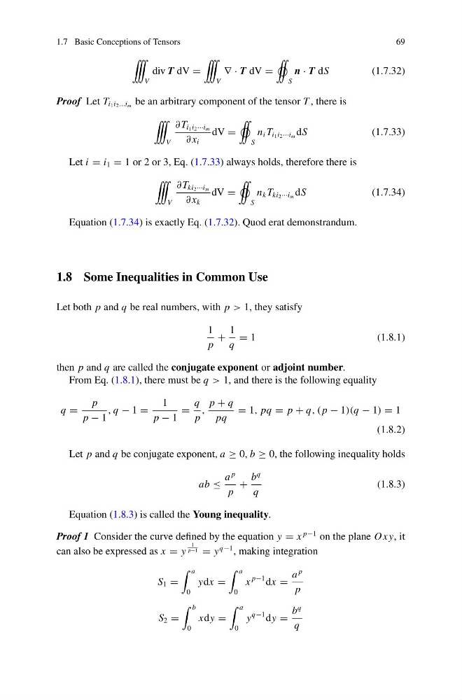
Proof Let T i 1 i 2 ...i m be an arbitrary component of the tensor T , there is
V
∂ T i 1 i 2 ···i m
∂ x i
dV =
S
n i T i 1 i 2 ···i m dS
(1.7.33)
Let i = i 1 = 1 or 2 or 3, Eq. (1.7.33) always holds, therefore there is
V
∂ T ki 2 ···i m
∂ x k
dV =
S
n k T ki 2 ···i m dS
(1.7.34)
Equation (1.7.34) is exactly Eq. (1.7.32). Quod erat demonstrandum.
1.8 Some Inequalities in Common Use
Let both p and q be real numbers, with p > 1, they satisfy
1
p
+
1
q
= 1
(1.8.1)
then p and q are called the conjugate exponent or adjoint number.
From Eq. (1.8.1), there must be q > 1, and there is the following equality
q =
p
p − 1
, q − 1 =
1
p − 1
=
q
p
,
p + q
pq
= 1, pq = p + q, (p − 1)(q − 1) = 1
(1.8.2)
Let p and q be conjugate exponent, a ≥ 0, b ≥ 0, the following inequality holds
ab ≤
a
p
p
+
b
q
q
(1.8.3)
Equation (1.8.3) is called the Young inequality.
Proof 1 Consider the curve defined by the equation y = x
p−1 on the plane Ox y, it
can also be expressed as x = y
1
p−1 = y
q−1 , making integration
S 1 =
a
0
ydx =
a
0
x
p−1 dx =
a
p
p
S 2 =
b
0
xdy =
a
0
y
q−1 dy =
b
q
q
69
V
div T dV =
V
∇ · T dV =
S
n · T dS
(1.7.32)
Proof Let T i 1 i 2 ...i m be an arbitrary component of the tensor T , there is
V
∂ T i 1 i 2 ···i m
∂ x i
dV =
S
n i T i 1 i 2 ···i m dS
(1.7.33)
Let i = i 1 = 1 or 2 or 3, Eq. (1.7.33) always holds, therefore there is
V
∂ T ki 2 ···i m
∂ x k
dV =
S
n k T ki 2 ···i m dS
(1.7.34)
Equation (1.7.34) is exactly Eq. (1.7.32). Quod erat demonstrandum.
1.8 Some Inequalities in Common Use
Let both p and q be real numbers, with p > 1, they satisfy
1
p
+
1
q
= 1
(1.8.1)
then p and q are called the conjugate exponent or adjoint number.
From Eq. (1.8.1), there must be q > 1, and there is the following equality
q =
p
p − 1
, q − 1 =
1
p − 1
=
q
p
,
p + q
pq
= 1, pq = p + q, (p − 1)(q − 1) = 1
(1.8.2)
Let p and q be conjugate exponent, a ≥ 0, b ≥ 0, the following inequality holds
ab ≤
a
p
p
+
b
q
q
(1.8.3)
Equation (1.8.3) is called the Young inequality.
Proof 1 Consider the curve defined by the equation y = x
p−1 on the plane Ox y, it
can also be expressed as x = y
1
p−1 = y
q−1 , making integration
S 1 =
a
0
ydx =
a
0
x
p−1 dx =
a
p
p
S 2 =
b
0
xdy =
a
0
y
q−1 dy =
b
q
q