Appendix: All Solutions to the Problems
809
From the boundary conditions u(0) = 0, u
(0) = 1, we get d 1 +d 2 = 0, d 1 −d 2 =
1, and we solve for d 1 =
1
2
, d 2 = −
1
2
. Thus u(x) =
e
x −e
−x
2
= sinh x.
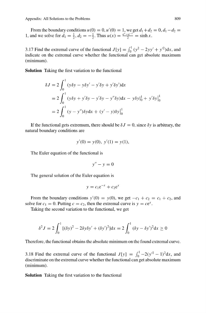
3.17 Find the extremal curve of the functional J [y] =
1
0 (y
2
− 2yy
+ y
2
)dx, and
indicate on the extremal curve whether the functional can get absolute maximum
(minimum).
Solution Taking the first variation to the functional
δ J = 2
1
0
(yδy − yδy
− y
δy + y
δy
)dx
= 2
1
0
(yδy + y
δy − y
δy − y
δy)dx − yδy|
1
0 + y
δy
1
0
= 2
1
0
(y − y
)δydx + (y
− y)δy
1
0
If the functional gets extremum, there should be δ J = 0, since δy is arbitrary, the
natural boundary conditions are
y
(0) = y(0), y
(1) = y(1),
The Euler equation of the functional is
y
− y = 0
The general solution of the Euler equation is
y = c 1 e
−x
+ c 2 e
x
From the boundary conditions y
(0) = y(0), we get −c 1 + c 2 = c 1 + c 2 , and
solve for c 1 = 0. Putting c = c 2 , then the extremal curve is y = ce
x .
Taking the second variation to the functional, we get
δ
2 J = 2
1
0
[(δy)
2
− 2δyδy
+ (δy
)
2
]dx = 2
1
0
(δy − δy
)
2 dx ≥ 0
Therefore, the functional obtains the absolute minimum on the found extremal curve.
3.18 Find the extremal curve of the functional J [y] =
1
0 −2(y
2
− 1)
2 dx, and
discriminate on the extremal curve whether the functional can get absolute maximum
(minimum).
Solution Taking the first variation to the functional