808
Appendix: All Solutions to the Problems
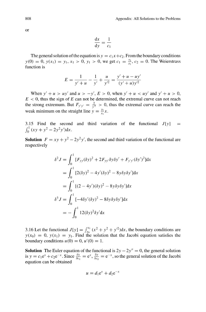
or
dx
dy
=
1
c 1
The general solution of the equation is y = c 1 x +c 2 . From the boundary conditions
y(0) = 0, y(x 1 ) = y 1 , x 1 > 0, y 1 > 0, we get c 1 =
y 1
x 1
, c 2 = 0. The Weierstrass
function is
E =
1
y + u
−
1
y +
u
y 2 =
y
+ u − uy
(y + u)y 2
When y
+ u > uy
and u > −y
, E > 0, when y
+ u < uy
and y
+ u > 0,
E < 0, thus the sign of E can not be determined, the extremal curve can not reach
the strong extremum. But F y y =
2
y 3 > 0, thus the extremal curve can reach the
weak minimum on the straight line y =
y 1
x 1
x.
3.15 Find the second and third variation of the functional J [y] =
1
0 (x y + y
2
− 2y
2 y
)dx.
Solution F = x y + y
2
− 2y
2 y
, the second and third variation of the functional are
respectively
δ
2 J =
1
0
[F yy (δy)
2
+ 2F yy δyδy
+ F y y (δy
)
2
]dx
=
1
0
[2(δy)
2
− 4y
(δy)
2
− 8yδyδy
]dx
=
1
0
[(2 − 4y
)(δy)
2
− 8yδyδy
]dx
δ
3 J =
1
0
[−4δy
(δy)
2
− 8δyδyδy
]dx
= −
1
0
12(δy)
2
δy
dx
3.16 Let the functional J [y] =
x 1
x 0
(x
2
+ y
2
+ y
2
)dx, the boundary conditions are
y(x 0 ) = 0, y(x 1 ) = y 1 . Find the solution that the Jacobi equation satisfies the
boundary conditions u(0) = 0, u
(0) = 1.
Solution The Euler equation of the functional is 2y − 2y
= 0, the general solution
is y = c 1 e
x
+ c 2 e
−x . Since
∂ y
∂c 1
= e
x ,
∂ y
∂c 2
= e
−x , so the general solution of the Jacobi
equation can be obtained
u = d 1 e
x
+ d 2 e
−x