688
10 Variational Problems of Functionals with Vector, Tensor …
∂ F
∂ A × ∇
n
· δ A × ∇ = ∇ ·
∂ F
∂ A × ∇
(n − 1)·
× δ A
+
∂ F
∂ A × ∇
× ∇
n
· δ A
(10.6.10)
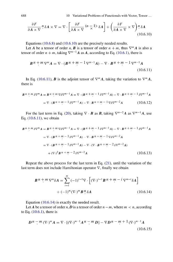
Equations (10.6.8) and (10.6.10) are the precisely needed results.
Let A be a tensor of order n, B is a tensor of order n + m, thus ∇
m A is also a
tensor of order n + m, taking ∇
m−1 A as A, according to Eq. (10.6.1), there is
B n + m
· ∇
m A = ∇ · (B n + m − 1
·
∇
m−1 A) − ∇ · B n + m − 1
·
∇
m−1 A
(10.6.11)
In Eq. (10.6.11), B is the adjoint tensor of ∇
m A, taking the variation to ∇
m A,
there is
B n + m
· δ∇ m A = B n + m
· ∇δ∇ m−1 A = ∇ · (B n + m − 1
·
δ∇ m−1 A) − ∇ · B n + m − 1
·
δ∇ m−1 A
= ∇ · (B n + m − 1
·
δ∇ m−1 A) − ∇ · B n + m − 1
·
∇δ∇ m−2 A
(10.6.12)
For the last term in Eq. (20), taking ∇ · B as B, taking ∇
m−2 A as ∇
m−1 A, use
Eq. (10.6.11), we obtain
B n + m
· δ∇ m A = B n + m
· ∇δ∇ m−1 A = ∇ · (B n + m − 1
·
δ∇ m−1 A) − ∇ · B n + m − 1
·
δ∇ m−1 A
= ∇ · (B n + m − 1
·
δ∇ m−1 A) − ∇ · B n + m − 1
·
∇δ∇ m−2 A
= ∇ · (B n + m − 1
·
δ∇ m−1 A) − ∇ · (∇ · B n + m − 2
·
δ∇ m−2 A)
+ (∇·) 2 B n + m − 2
·
δ∇ m−2 A
(10.6.13)
Repeat the above process for the last term in Eq. (21), until the variation of the
last term does not include Hamiltonian operator ∇, finally we obtain
B n + m
· ∇
m
δ A =
m
i=1
(−1)
i−1
∇ ·
(∇·)
i−1 B n + m − i
·
∇
m−i
δ A
+ (−1)
m
(∇·)
m B n
· δ A
(10.6.14)
Equation (10.6.14) is exactly the needed result.
Let A be a tensor of order n, D is a tensor of order n − m, where m < n, according
to Eq. (10.6.1), there is
D n − m
· (∇·)
m A = ∇ · [(∇·)
m−1 A n − m
· D] − ∇ D n − m + 1
·
(∇·)
m−1 A
(10.6.15)