

9.10 The Maupertuis-Lagrange Principle of Least Action
593
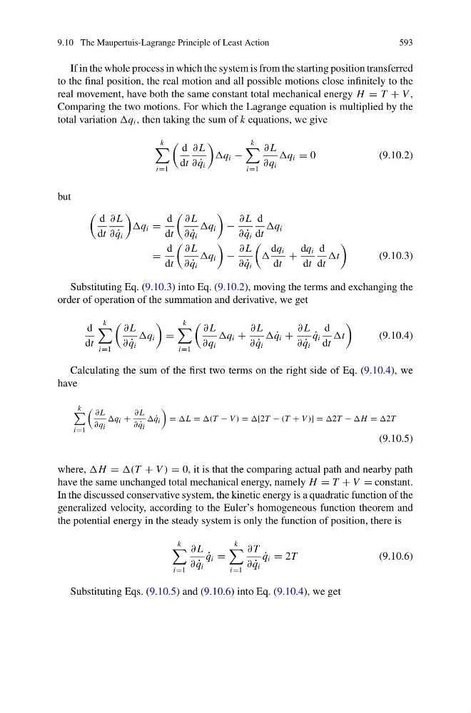
If in the whole process in which the system is from the starting position transferred
to the final position, the real motion and all possible motions close infinitely to the
real movement, have both the same constant total mechanical energy H = T + V ,
Comparing the two motions. For which the Lagrange equation is multiplied by the
total variation q i , then taking the sum of k equations, we give
k
i=1
d
dt
∂ L
∂ ˙
q i
q i −
k
i=1
∂ L
∂q i
q i = 0
(9.10.2)
but
d
dt
∂ L
∂ ˙
q i
q i =
d
dt
∂ L
∂ ˙
q i
q i
−
∂ L
∂ ˙
q i
d
dt
q i
=
d
dt
∂ L
∂ ˙
q i
q i
−
∂ L
∂ ˙
q i
dq i
dt
+
dq i
dt
d
dt
t
(9.10.3)
Substituting Eq. (9.10.3) into Eq. (9.10.2), moving the terms and exchanging the
order of operation of the summation and derivative, we get
d
dt
k
i=1
∂ L
∂ ˙
q i
q i
=
k
i=1
∂ L
∂q i
q i +
∂ L
∂ ˙
q i
˙
q i +
∂ L
∂ ˙
q i
˙
q i
d
dt
t
(9.10.4)
Calculating the sum of the first two terms on the right side of Eq. (9.10.4), we
have
k
i=1
∂ L
∂q i
q i +
∂ L
∂ ˙
q i
˙
q i
= L = (T − V ) = [2T − (T + V )] = 2T − H = 2T
(9.10.5)
where, H = (T + V ) = 0, it is that the comparing actual path and nearby path
have the same unchanged total mechanical energy, namely H = T + V = constant.
In the discussed conservative system, the kinetic energy is a quadratic function of the
generalized velocity, according to the Euler’s homogeneous function theorem and
the potential energy in the steady system is only the function of position, there is
k
i=1
∂ L
∂ ˙
q i
˙
q i =
k
i=1
∂ T
∂ ˙
q i
˙
q i = 2T
(9.10.6)
Substituting Eqs. (9.10.5) and (9.10.6) into Eq. (9.10.4), we get
593
If in the whole process in which the system is from the starting position transferred
to the final position, the real motion and all possible motions close infinitely to the
real movement, have both the same constant total mechanical energy H = T + V ,
Comparing the two motions. For which the Lagrange equation is multiplied by the
total variation q i , then taking the sum of k equations, we give
k
i=1
d
dt
∂ L
∂ ˙
q i
q i −
k
i=1
∂ L
∂q i
q i = 0
(9.10.2)
but
d
dt
∂ L
∂ ˙
q i
q i =
d
dt
∂ L
∂ ˙
q i
q i
−
∂ L
∂ ˙
q i
d
dt
q i
=
d
dt
∂ L
∂ ˙
q i
q i
−
∂ L
∂ ˙
q i
dq i
dt
+
dq i
dt
d
dt
t
(9.10.3)
Substituting Eq. (9.10.3) into Eq. (9.10.2), moving the terms and exchanging the
order of operation of the summation and derivative, we get
d
dt
k
i=1
∂ L
∂ ˙
q i
q i
=
k
i=1
∂ L
∂q i
q i +
∂ L
∂ ˙
q i
˙
q i +
∂ L
∂ ˙
q i
˙
q i
d
dt
t
(9.10.4)
Calculating the sum of the first two terms on the right side of Eq. (9.10.4), we
have
k
i=1
∂ L
∂q i
q i +
∂ L
∂ ˙
q i
˙
q i
= L = (T − V ) = [2T − (T + V )] = 2T − H = 2T
(9.10.5)
where, H = (T + V ) = 0, it is that the comparing actual path and nearby path
have the same unchanged total mechanical energy, namely H = T + V = constant.
In the discussed conservative system, the kinetic energy is a quadratic function of the
generalized velocity, according to the Euler’s homogeneous function theorem and
the potential energy in the steady system is only the function of position, there is
k
i=1
∂ L
∂ ˙
q i
˙
q i =
k
i=1
∂ T
∂ ˙
q i
˙
q i = 2T
(9.10.6)
Substituting Eqs. (9.10.5) and (9.10.6) into Eq. (9.10.4), we get