

570
9 Variational Principles in Mechanics and Their Applications
E I y =
qx
4
24
+ c 1 x
3
+ c 2 x
2
+ c 3 x + c 4
(11)
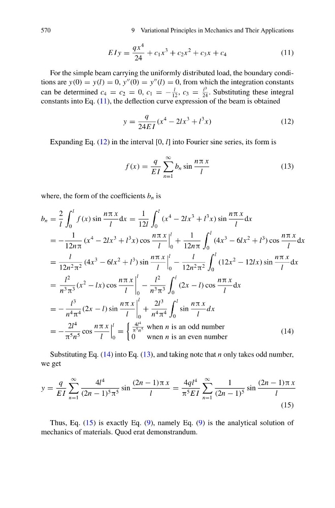
For the simple beam carrying the uniformly distributed load, the boundary conditions are y(0) = y(l) = 0, y
(0) = y
(l) = 0, from which the integration constants
can be determined c 4 = c 2 = 0, c 1 = −
l
12
, c 3 =
l
3
24
. Substituting these integral
constants into Eq. (11), the deflection curve expression of the beam is obtained
y =
q
24E I
(x
4
− 2lx
3
+ l
3 x)
(12)
Expanding Eq. (12) in the interval [0, l] into Fourier sine series, its form is
f (x) =
q
E I
∞
n=1
b n sin
nπ x
l
(13)
where, the form of the coefficients b n is
b n =
2
l
l
0
f (x) sin
nπ x
l
dx =
1
12l
l
0
(x
4
− 2lx
3
+ l
3 x) sin
nπ x
l
dx
= −
1
12nπ
(x
4
− 2lx
3
+ l
3 x) cos
nπ x
l
l
0
+
1
12nπ
l
0
(4x
3
− 6lx
2
+ l
3
) cos
nπ x
l
dx
=
l
12n 2 π 2 (4x
3
− 6lx
2
+ l
3
) sin
nπ x
l
l
0
−
l
12n 2 π 2
l
0
(12x
2
− 12lx) sin
nπ x
l
dx
=
l
2
n 3 π 3 (x
2
− lx) cos
nπ x
l
l
0
−
l
2
n 3 π 3
l
0
(2x − l) cos
nπ x
l
dx
= −
l
3
n 4 π 4 (2x − l) sin
nπ x
l
l
0
+
2l
3
n 4 π 4
l
0
sin
nπ x
l
dx
= −
2l
4
π 5 n 5 cos
nπ x
l
l
0
=
4l
4
π 5 n 5 when n is an odd number
0 wnen n is an even number
(14)
Substituting Eq. (14) into Eq. (13), and taking note that n only takes odd number,
we get
y =
q
E I
∞
n=1
4l
4
(2n − 1) 5 π 5 sin
(2n − 1)π x
l
=
4ql
4
π 5 E I
∞
n=1
1
(2n − 1) 5 sin
(2n − 1)π x
l
(15)
Thus, Eq. (15) is exactly Eq. (9), namely Eq. (9) is the analytical solution of
mechanics of materials. Quod erat demonstrandum.
9 Variational Principles in Mechanics and Their Applications
E I y =
qx
4
24
+ c 1 x
3
+ c 2 x
2
+ c 3 x + c 4
(11)
For the simple beam carrying the uniformly distributed load, the boundary conditions are y(0) = y(l) = 0, y
(0) = y
(l) = 0, from which the integration constants
can be determined c 4 = c 2 = 0, c 1 = −
l
12
, c 3 =
l
3
24
. Substituting these integral
constants into Eq. (11), the deflection curve expression of the beam is obtained
y =
q
24E I
(x
4
− 2lx
3
+ l
3 x)
(12)
Expanding Eq. (12) in the interval [0, l] into Fourier sine series, its form is
f (x) =
q
E I
∞
n=1
b n sin
nπ x
l
(13)
where, the form of the coefficients b n is
b n =
2
l
l
0
f (x) sin
nπ x
l
dx =
1
12l
l
0
(x
4
− 2lx
3
+ l
3 x) sin
nπ x
l
dx
= −
1
12nπ
(x
4
− 2lx
3
+ l
3 x) cos
nπ x
l
l
0
+
1
12nπ
l
0
(4x
3
− 6lx
2
+ l
3
) cos
nπ x
l
dx
=
l
12n 2 π 2 (4x
3
− 6lx
2
+ l
3
) sin
nπ x
l
l
0
−
l
12n 2 π 2
l
0
(12x
2
− 12lx) sin
nπ x
l
dx
=
l
2
n 3 π 3 (x
2
− lx) cos
nπ x
l
l
0
−
l
2
n 3 π 3
l
0
(2x − l) cos
nπ x
l
dx
= −
l
3
n 4 π 4 (2x − l) sin
nπ x
l
l
0
+
2l
3
n 4 π 4
l
0
sin
nπ x
l
dx
= −
2l
4
π 5 n 5 cos
nπ x
l
l
0
=
4l
4
π 5 n 5 when n is an odd number
0 wnen n is an even number
(14)
Substituting Eq. (14) into Eq. (13), and taking note that n only takes odd number,
we get
y =
q
E I
∞
n=1
4l
4
(2n − 1) 5 π 5 sin
(2n − 1)π x
l
=
4ql
4
π 5 E I
∞
n=1
1
(2n − 1) 5 sin
(2n − 1)π x
l
(15)
Thus, Eq. (15) is exactly Eq. (9), namely Eq. (9) is the analytical solution of
mechanics of materials. Quod erat demonstrandum.