

8.7 Eigenvalues and Eigenfunctions of Operator Equations
493
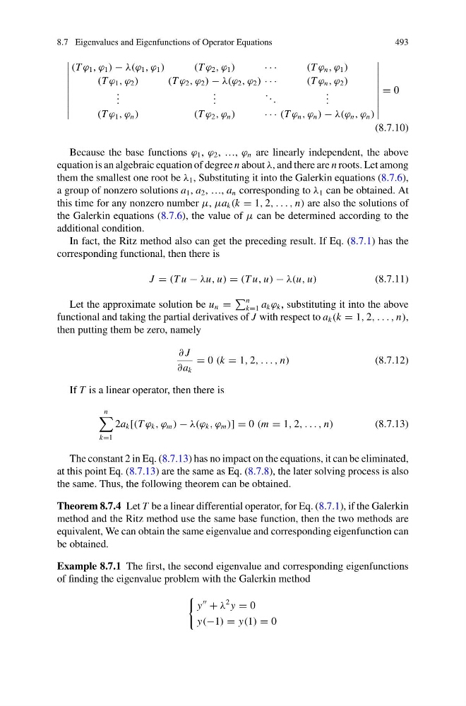
(T ϕ 1 , ϕ 1 ) − λ(ϕ 1 , ϕ 1 )
(T ϕ 2 , ϕ 1 )
· · ·
(T ϕ n , ϕ 1 )
(T ϕ 1 , ϕ 2 )
(T ϕ 2 , ϕ 2 ) − λ(ϕ 2 , ϕ 2 ) · · ·
(T ϕ n , ϕ 2 )
. . .
. . .
. . .
. . .
(T ϕ 1 , ϕ n )
( T ϕ 2 , ϕ n )
· · · (T ϕ n , ϕ n ) − λ(ϕ n , ϕ n )
= 0
(8.7.10)
Because the base functions ϕ 1 , ϕ 2 , …, ϕ n are linearly independent, the above
equation is an algebraic equation of degree n about λ, and there are n roots. Let among
them the smallest one root be λ 1 , Substituting it into the Galerkin equations (8.7.6),
a group of nonzero solutions a 1 , a 2 , …, a n corresponding to λ 1 can be obtained. At
this time for any nonzero number μ, μa k (k = 1, 2, . . . , n) are also the solutions of
the Galerkin equations (8.7.6), the value of μ can be determined according to the
additional condition.
In fact, the Ritz method also can get the preceding result. If Eq. (8.7.1) has the
corresponding functional, then there is
J = (T u − λu, u) = (T u, u) − λ(u, u)
(8.7.11)
Let the approximate solution be u n =
n
k=1 a k ϕ k , substituting it into the above
functional and taking the partial derivatives of J with respect to a k (k = 1, 2, . . . , n),
then putting them be zero, namely
∂ J
∂a k
= 0 (k = 1, 2, . . . , n)
(8.7.12)
If T is a linear operator, then there is
n
k=1
2a k [(T ϕ k , ϕ m ) − λ(ϕ k , ϕ m )] = 0 (m = 1, 2, . . . , n)
(8.7.13)
The constant 2 in Eq. (8.7.13) has no impact on the equations, it can be eliminated,
at this point Eq. (8.7.13) are the same as Eq. (8.7.8), the later solving process is also
the same. Thus, the following theorem can be obtained.
Theorem 8.7.4 Let T be a linear differential operator, for Eq. (8.7.1), if the Galerkin
method and the Ritz method use the same base function, then the two methods are
equivalent, We can obtain the same eigenvalue and corresponding eigenfunction can
be obtained.
Example 8.7.1 The first, the second eigenvalue and corresponding eigenfunctions
of finding the eigenvalue problem with the Galerkin method
y
+ λ
2 y = 0
y(−1) = y(1) = 0
493
(T ϕ 1 , ϕ 1 ) − λ(ϕ 1 , ϕ 1 )
(T ϕ 2 , ϕ 1 )
· · ·
(T ϕ n , ϕ 1 )
(T ϕ 1 , ϕ 2 )
(T ϕ 2 , ϕ 2 ) − λ(ϕ 2 , ϕ 2 ) · · ·
(T ϕ n , ϕ 2 )
. . .
. . .
. . .
. . .
(T ϕ 1 , ϕ n )
( T ϕ 2 , ϕ n )
· · · (T ϕ n , ϕ n ) − λ(ϕ n , ϕ n )
= 0
(8.7.10)
Because the base functions ϕ 1 , ϕ 2 , …, ϕ n are linearly independent, the above
equation is an algebraic equation of degree n about λ, and there are n roots. Let among
them the smallest one root be λ 1 , Substituting it into the Galerkin equations (8.7.6),
a group of nonzero solutions a 1 , a 2 , …, a n corresponding to λ 1 can be obtained. At
this time for any nonzero number μ, μa k (k = 1, 2, . . . , n) are also the solutions of
the Galerkin equations (8.7.6), the value of μ can be determined according to the
additional condition.
In fact, the Ritz method also can get the preceding result. If Eq. (8.7.1) has the
corresponding functional, then there is
J = (T u − λu, u) = (T u, u) − λ(u, u)
(8.7.11)
Let the approximate solution be u n =
n
k=1 a k ϕ k , substituting it into the above
functional and taking the partial derivatives of J with respect to a k (k = 1, 2, . . . , n),
then putting them be zero, namely
∂ J
∂a k
= 0 (k = 1, 2, . . . , n)
(8.7.12)
If T is a linear operator, then there is
n
k=1
2a k [(T ϕ k , ϕ m ) − λ(ϕ k , ϕ m )] = 0 (m = 1, 2, . . . , n)
(8.7.13)
The constant 2 in Eq. (8.7.13) has no impact on the equations, it can be eliminated,
at this point Eq. (8.7.13) are the same as Eq. (8.7.8), the later solving process is also
the same. Thus, the following theorem can be obtained.
Theorem 8.7.4 Let T be a linear differential operator, for Eq. (8.7.1), if the Galerkin
method and the Ritz method use the same base function, then the two methods are
equivalent, We can obtain the same eigenvalue and corresponding eigenfunction can
be obtained.
Example 8.7.1 The first, the second eigenvalue and corresponding eigenfunctions
of finding the eigenvalue problem with the Galerkin method
y
+ λ
2 y = 0
y(−1) = y(1) = 0