

492
8 Direct Methods of Variational Problems
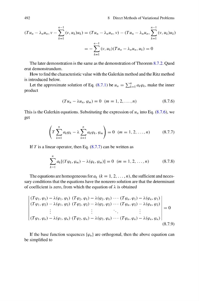
(T u n − λ n u n , v −
n−1
k=1
(v, u k )u k ) = (T u n − λ n u n , v) − (T u n − λ n u n ,
n−1
k=1
(v, u k )u k )
= −
n−1
k=1
(v, u k )(T u n − λ n u n , u k ) = 0
The later demonstration is the same as the demonstration of Theorem 8.7.2. Quod
erat demonstrandum.
How to find the characteristic value with the Galerkin method and the Ritz method
is introduced below.
Let the approximate solution of Eq. (8.7.1) be u n =
n
k=1 a k ϕ k , make the inner
product
(T u n − λu n , ϕ m ) = 0 (m = 1, 2, . . . , n)
(8.7.6)
This is the Galerkin equations. Substituting the expression of u n into Eq. (8.7.6), we
get
T
n
k=1
a k ϕ k − λ
n
k=1
a k ϕ k , ϕ m
= 0 (m = 1, 2, . . . , n)
(8.7.7)
If T is a linear operator, then Eq. (8.7.7) can be written as
n
k=1
a k [(T ϕ k , ϕ m ) − λ(ϕ k , ϕ m )] = 0 (m = 1, 2, . . . , n)
(8.7.8)
The equations are homogeneous for a k (k = 1, 2, . . . , n), the sufficient and necessary conditions that the equations have the nonzero solution are that the determinant
of coefficient is zero, from which the equation of λ is obtained
(T ϕ 1 , ϕ 1 ) − λ(ϕ 1 , ϕ 1 ) (T ϕ 2 , ϕ 1 ) − λ(ϕ 2 , ϕ 1 ) · · · (T ϕ n , ϕ 1 ) − λ(ϕ n , ϕ 1 )
(T ϕ 1 , ϕ 2 ) − λ(ϕ 1 , ϕ 2 ) (T ϕ 2 , ϕ 2 ) − λ(ϕ 2 , ϕ 2 ) · · · (T ϕ n , ϕ 2 ) − λ(ϕ n , ϕ 2 )
. . .
. . .
. . .
. . .
(T ϕ 1 , ϕ n ) − λ(ϕ 1 , ϕ n ) (T ϕ 2 , ϕ n ) − λ(ϕ 2 , ϕ n ) · · · (T ϕ n , ϕ n ) − λ(ϕ n , ϕ n )
= 0
(8.7.9)
If the base function sequences {ϕ n } are orthogonal, then the above equation can
be simplified to
8 Direct Methods of Variational Problems
(T u n − λ n u n , v −
n−1
k=1
(v, u k )u k ) = (T u n − λ n u n , v) − (T u n − λ n u n ,
n−1
k=1
(v, u k )u k )
= −
n−1
k=1
(v, u k )(T u n − λ n u n , u k ) = 0
The later demonstration is the same as the demonstration of Theorem 8.7.2. Quod
erat demonstrandum.
How to find the characteristic value with the Galerkin method and the Ritz method
is introduced below.
Let the approximate solution of Eq. (8.7.1) be u n =
n
k=1 a k ϕ k , make the inner
product
(T u n − λu n , ϕ m ) = 0 (m = 1, 2, . . . , n)
(8.7.6)
This is the Galerkin equations. Substituting the expression of u n into Eq. (8.7.6), we
get
T
n
k=1
a k ϕ k − λ
n
k=1
a k ϕ k , ϕ m
= 0 (m = 1, 2, . . . , n)
(8.7.7)
If T is a linear operator, then Eq. (8.7.7) can be written as
n
k=1
a k [(T ϕ k , ϕ m ) − λ(ϕ k , ϕ m )] = 0 (m = 1, 2, . . . , n)
(8.7.8)
The equations are homogeneous for a k (k = 1, 2, . . . , n), the sufficient and necessary conditions that the equations have the nonzero solution are that the determinant
of coefficient is zero, from which the equation of λ is obtained
(T ϕ 1 , ϕ 1 ) − λ(ϕ 1 , ϕ 1 ) (T ϕ 2 , ϕ 1 ) − λ(ϕ 2 , ϕ 1 ) · · · (T ϕ n , ϕ 1 ) − λ(ϕ n , ϕ 1 )
(T ϕ 1 , ϕ 2 ) − λ(ϕ 1 , ϕ 2 ) (T ϕ 2 , ϕ 2 ) − λ(ϕ 2 , ϕ 2 ) · · · (T ϕ n , ϕ 2 ) − λ(ϕ n , ϕ 2 )
. . .
. . .
. . .
. . .
(T ϕ 1 , ϕ n ) − λ(ϕ 1 , ϕ n ) (T ϕ 2 , ϕ n ) − λ(ϕ 2 , ϕ n ) · · · (T ϕ n , ϕ n ) − λ(ϕ n , ϕ n )
= 0
(8.7.9)
If the base function sequences {ϕ n } are orthogonal, then the above equation can
be simplified to