

494
8 Direct Methods of Variational Problems
and comparing to the eigenvalues of the analytical solution.
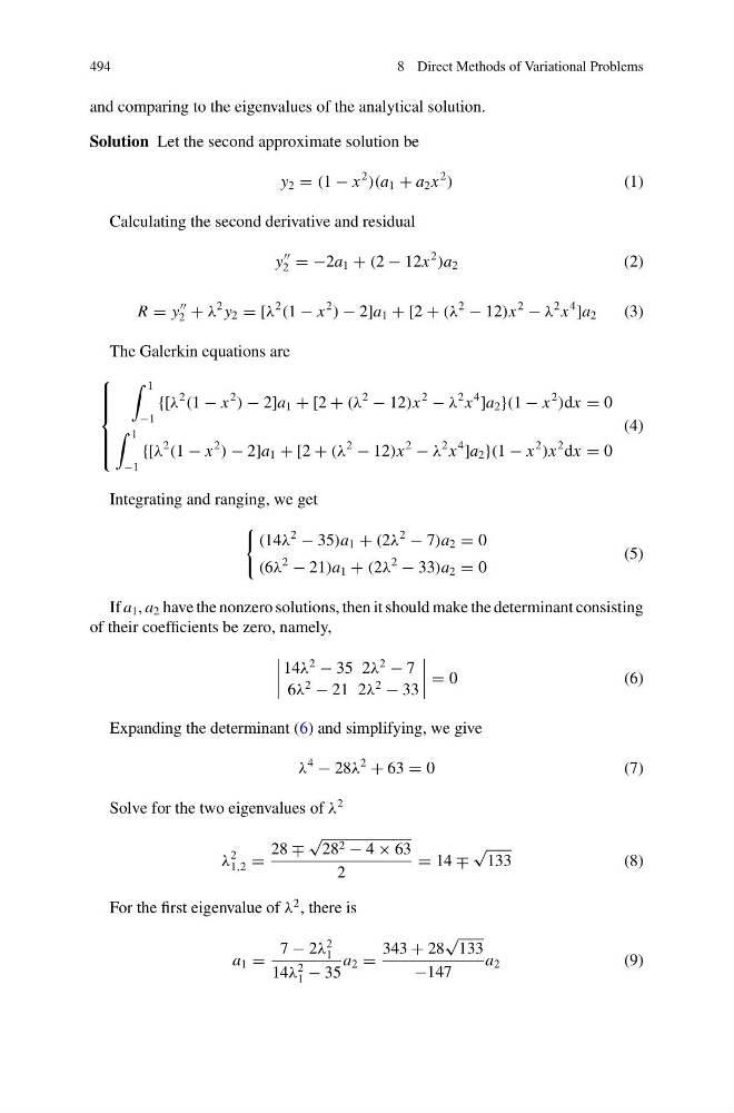
Solution Let the second approximate solution be
y 2 = (1 − x
2
)(a 1 + a 2 x
2
)
(1)
Calculating the second derivative and residual
y
2 = −2a 1 + (2 − 12x
2
)a 2
(2)
R = y
2 + λ
2 y 2 = [λ
2
(1 − x
2
) − 2]a 1 + [2 + (λ
2
− 12)x
2
− λ
2 x
4
]a 2
(3)
The Galerkin equations are
⎧
⎪ ⎪ ⎪ ⎨
⎪ ⎪ ⎪ ⎩
1
−1
{[λ
2
(1 − x
2
) − 2]a 1 + [2 + (λ
2
− 12)x
2
− λ
2 x
4
]a 2 }(1 − x
2
)dx = 0
1
−1
{[λ
2
(1 − x
2
) − 2]a 1 + [2 + (λ
2
− 12)x
2
− λ
2 x
4
]a 2 }(1 − x
2
)x
2 dx = 0
(4)
Integrating and ranging, we get
(14λ
2
− 35)a 1 + (2λ
2
− 7)a 2 = 0
(6λ
2
− 21)a 1 + (2λ
2
− 33)a 2 = 0
(5)
If a 1 , a 2 have the nonzero solutions, then it should make the determinant consisting
of their coefficients be zero, namely,
14λ
2
− 35 2λ
2
− 7
6λ
2
− 21 2λ
2
− 33
= 0
( 6 )
Expanding the determinant (6) and simplifying, we give
λ
4
− 28λ
2
+ 63 = 0
( 7 )
Solve for the two eigenvalues of λ
2
λ
2
1,2 =
28 ∓
√
28 2 − 4 × 63
2
= 14 ∓
√
133
(8)
For the first eigenvalue of λ
2 , there is
a 1 =
7 − 2λ
2
1
14λ
2
1 − 35
a 2 =
343 + 28
√
133
−147
a 2
(9)
8 Direct Methods of Variational Problems
and comparing to the eigenvalues of the analytical solution.
Solution Let the second approximate solution be
y 2 = (1 − x
2
)(a 1 + a 2 x
2
)
(1)
Calculating the second derivative and residual
y
2 = −2a 1 + (2 − 12x
2
)a 2
(2)
R = y
2 + λ
2 y 2 = [λ
2
(1 − x
2
) − 2]a 1 + [2 + (λ
2
− 12)x
2
− λ
2 x
4
]a 2
(3)
The Galerkin equations are
⎧
⎪ ⎪ ⎪ ⎨
⎪ ⎪ ⎪ ⎩
1
−1
{[λ
2
(1 − x
2
) − 2]a 1 + [2 + (λ
2
− 12)x
2
− λ
2 x
4
]a 2 }(1 − x
2
)dx = 0
1
−1
{[λ
2
(1 − x
2
) − 2]a 1 + [2 + (λ
2
− 12)x
2
− λ
2 x
4
]a 2 }(1 − x
2
)x
2 dx = 0
(4)
Integrating and ranging, we get
(14λ
2
− 35)a 1 + (2λ
2
− 7)a 2 = 0
(6λ
2
− 21)a 1 + (2λ
2
− 33)a 2 = 0
(5)
If a 1 , a 2 have the nonzero solutions, then it should make the determinant consisting
of their coefficients be zero, namely,
14λ
2
− 35 2λ
2
− 7
6λ
2
− 21 2λ
2
− 33
= 0
( 6 )
Expanding the determinant (6) and simplifying, we give
λ
4
− 28λ
2
+ 63 = 0
( 7 )
Solve for the two eigenvalues of λ
2
λ
2
1,2 =
28 ∓
√
28 2 − 4 × 63
2
= 14 ∓
√
133
(8)
For the first eigenvalue of λ
2 , there is
a 1 =
7 − 2λ
2
1
14λ
2
1 − 35
a 2 =
343 + 28
√
133
−147
a 2
(9)