

8.6 The Least Square Method
487
y n (x) =
n
k=1
a k (1 − x)x
k
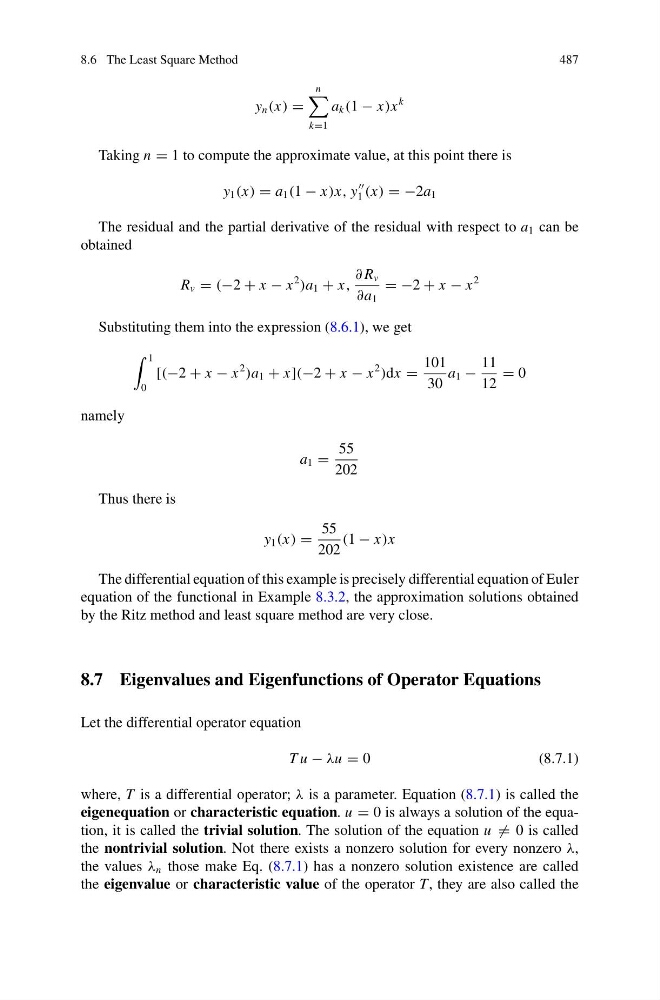
Taking n = 1 to compute the approximate value, at this point there is
y 1 (x) = a 1 (1 − x)x, y
1 (x) = −2a 1
The residual and the partial derivative of the residual with respect to a 1 can be
obtained
R v = (−2 + x − x
2
)a 1 + x,
∂ R v
∂a 1
= −2 + x − x
2
Substituting them into the expression (8.6.1), we get
1
0
[(−2 + x − x
2
)a 1 + x](−2 + x − x
2
)dx =
101
30
a 1 −
11
12
= 0
namely
a 1 =
55
202
Thus there is
y 1 (x) =
55
202
(1 − x)x
The differential equation of this example is precisely differential equation of Euler
equation of the functional in Example 8.3.2, the approximation solutions obtained
by the Ritz method and least square method are very close.
8.7 Eigenvalues and Eigenfunctions of Operator Equations
Let the differential operator equation
T u − λu = 0
(8.7.1)
where, T is a differential operator; λ is a parameter. Equation (8.7.1) is called the
eigenequation or characteristic equation. u = 0 is always a solution of the equation, it is called the trivial solution. The solution of the equation u = 0 is called
the nontrivial solution. Not there exists a nonzero solution for every nonzero λ,
the values λ n those make Eq. (8.7.1) has a nonzero solution existence are called
the eigenvalue or characteristic value of the operator T, they are also called the
487
y n (x) =
n
k=1
a k (1 − x)x
k
Taking n = 1 to compute the approximate value, at this point there is
y 1 (x) = a 1 (1 − x)x, y
1 (x) = −2a 1
The residual and the partial derivative of the residual with respect to a 1 can be
obtained
R v = (−2 + x − x
2
)a 1 + x,
∂ R v
∂a 1
= −2 + x − x
2
Substituting them into the expression (8.6.1), we get
1
0
[(−2 + x − x
2
)a 1 + x](−2 + x − x
2
)dx =
101
30
a 1 −
11
12
= 0
namely
a 1 =
55
202
Thus there is
y 1 (x) =
55
202
(1 − x)x
The differential equation of this example is precisely differential equation of Euler
equation of the functional in Example 8.3.2, the approximation solutions obtained
by the Ritz method and least square method are very close.
8.7 Eigenvalues and Eigenfunctions of Operator Equations
Let the differential operator equation
T u − λu = 0
(8.7.1)
where, T is a differential operator; λ is a parameter. Equation (8.7.1) is called the
eigenequation or characteristic equation. u = 0 is always a solution of the equation, it is called the trivial solution. The solution of the equation u = 0 is called
the nontrivial solution. Not there exists a nonzero solution for every nonzero λ,
the values λ n those make Eq. (8.7.1) has a nonzero solution existence are called
the eigenvalue or characteristic value of the operator T, they are also called the