

8.2 The Euler Finite Difference Method
461
ϕ(y 1 , y 2 , y 3 , y 4 ) =
y 1
x
2 +
y 2 − y 1
x
2
+
y 3 − y 2
x
2
+
y 4 − y 3
x
2
+
−y 4
x
2
+ y
2
1 + y
2
2 + y
2
3 + y
2
4 + 2((xy 1 + 2xy 2 + 3xy 3 + 4xy 4 )]x
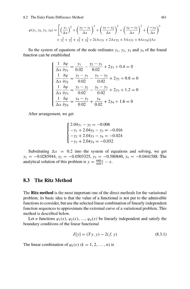
So the system of equations of the node ordinates y 1 , y 2 , y 3 and y 4 of the found
function can be established
⎧
⎪ ⎪ ⎪ ⎪ ⎪ ⎪ ⎪ ⎪ ⎪ ⎪ ⎪ ⎨
⎪ ⎪ ⎪ ⎪ ⎪ ⎪ ⎪ ⎪ ⎪ ⎪ ⎪ ⎩
1
x
∂ϕ
∂ y 1
=
y 1
0.02
−
y 2 − y 1
0.02
+ 2y 1 + 0.4 = 0
1
x
∂ϕ
∂ y 2
=
y 2 − y 1
0.02
−
y 3 − y 2
0.02
+ 2y 2 + 0.8 = 0
1
x
∂ϕ
∂ y 3
=
y 3 − y 2
0.02
−
y 4 − y 3
0.02
+ 2y 3 + 1.2 = 0
1
x
∂ϕ
∂ y 4
=
y 4 − y 3
0.02
+
y 4
0.02
+ 2y 4 + 1.6 = 0
After arrangement, we get
⎧
⎪ ⎪ ⎨
⎪ ⎪ ⎩
2.04y 1 − y 2 = −0.008
−y 1 + 2.04y 2 − y 3 = −0.016
−y 2 + 2.04y 3 − y 4 = −0.024
−y 3 + 2.04y 4 = −0.032
Substituting x = 0.2 into the system of equations and solving, we get
y 1 = −0.0285944, y 2 = −0.0503325, y 3 = −0.580840, y 4 = −0.0441588. The
analytical solution of this problem is y =
sinh x
sinh 1
− x.
8.3 The Ritz Method
The Ritz method is the most important one of the direct methods for the variational
problem, its basic idea is that the value of a functional is not put to the admissible
functions to consider, but use the selected linear combination of linearly independent
function sequences to approximate the extremal curve of a variational problem. This
method is described below.
Let n functions ϕ 1 (x), ϕ 2 (x), …, ϕ n (x) be linearly independent and satisfy the
boundary conditions of the linear functional
J [y] = (T y, y) − 2( f, y)
(8.3.1)
The linear combination of ϕ k (x) (k = 1, 2, . . . , n) is
461
ϕ(y 1 , y 2 , y 3 , y 4 ) =
y 1
x
2 +
y 2 − y 1
x
2
+
y 3 − y 2
x
2
+
y 4 − y 3
x
2
+
−y 4
x
2
+ y
2
1 + y
2
2 + y
2
3 + y
2
4 + 2((xy 1 + 2xy 2 + 3xy 3 + 4xy 4 )]x
So the system of equations of the node ordinates y 1 , y 2 , y 3 and y 4 of the found
function can be established
⎧
⎪ ⎪ ⎪ ⎪ ⎪ ⎪ ⎪ ⎪ ⎪ ⎪ ⎪ ⎨
⎪ ⎪ ⎪ ⎪ ⎪ ⎪ ⎪ ⎪ ⎪ ⎪ ⎪ ⎩
1
x
∂ϕ
∂ y 1
=
y 1
0.02
−
y 2 − y 1
0.02
+ 2y 1 + 0.4 = 0
1
x
∂ϕ
∂ y 2
=
y 2 − y 1
0.02
−
y 3 − y 2
0.02
+ 2y 2 + 0.8 = 0
1
x
∂ϕ
∂ y 3
=
y 3 − y 2
0.02
−
y 4 − y 3
0.02
+ 2y 3 + 1.2 = 0
1
x
∂ϕ
∂ y 4
=
y 4 − y 3
0.02
+
y 4
0.02
+ 2y 4 + 1.6 = 0
After arrangement, we get
⎧
⎪ ⎪ ⎨
⎪ ⎪ ⎩
2.04y 1 − y 2 = −0.008
−y 1 + 2.04y 2 − y 3 = −0.016
−y 2 + 2.04y 3 − y 4 = −0.024
−y 3 + 2.04y 4 = −0.032
Substituting x = 0.2 into the system of equations and solving, we get
y 1 = −0.0285944, y 2 = −0.0503325, y 3 = −0.580840, y 4 = −0.0441588. The
analytical solution of this problem is y =
sinh x
sinh 1
− x.
8.3 The Ritz Method
The Ritz method is the most important one of the direct methods for the variational
problem, its basic idea is that the value of a functional is not put to the admissible
functions to consider, but use the selected linear combination of linearly independent
function sequences to approximate the extremal curve of a variational problem. This
method is described below.
Let n functions ϕ 1 (x), ϕ 2 (x), …, ϕ n (x) be linearly independent and satisfy the
boundary conditions of the linear functional
J [y] = (T y, y) − 2( f, y)
(8.3.1)
The linear combination of ϕ k (x) (k = 1, 2, . . . , n) is