

460
8 Direct Methods of Variational Problems
F y
x i , y i ,
y i
x
−
F y
x i , y i ,
y i
x
− F y
x i−1 , y i−1 ,
y i−1
x
x
= 0
(8.2.8)
or
F y
x i , y i ,
y i
x
−
F y
i
x
= 0
(8.2.9)
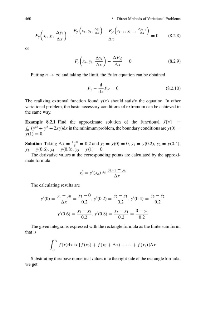
Putting n → ∞ and taking the limit, the Euler equation can be obtained
F y −
d
dx
F y = 0
(8.2.10)
The realizing extremal function found y(x) should satisfy the equation. In other
variational problem, the basic necessary conditions of extremum can be achieved in
the same way.
Example 8.2.1 Find the approximate solution of the functional J [y] =
1
0 (y
2
+ y
2
+ 2x y)dx in the minimum problem, the boundary conditions are y(0) =
y(1) = 0.
Solution Taking x =
1−0
5
= 0.2 and y 0 = y(0) = 0, y 1 = y(0.2), y 2 = y(0.4),
y 3 = y(0.6), y 4 = y(0.8), y 5 = y(1) = 0.
The derivative values at the corresponding points are calculated by the approximate formula
y
k = y
(x k ) ≈
y k+1 − y k
x
The calculating results are
y
(0) =
y 1 − y 0
x
=
y 1 − 0
0.2
, y
(0.2) =
y 2 − y 1
0.2
, y
(0.4) =
y 3 − y 2
0.2
y
(0.6) =
y 4 − y 3
0.2
, y
(0.8) =
y 5 − y 4
0.2
=
0 − y 4
0.2
The given integral is expressed with the rectangle formula as the finite sum form,
that is
x 1
x 0
f (x)dx ≈ [ f (x 0 ) + f (x 0 + x) + · · · + f (x 1 )]x
Substituting the above numerical values into the right side of the rectangle formula,
we get
8 Direct Methods of Variational Problems
F y
x i , y i ,
y i
x
−
F y
x i , y i ,
y i
x
− F y
x i−1 , y i−1 ,
y i−1
x
x
= 0
(8.2.8)
or
F y
x i , y i ,
y i
x
−
F y
i
x
= 0
(8.2.9)
Putting n → ∞ and taking the limit, the Euler equation can be obtained
F y −
d
dx
F y = 0
(8.2.10)
The realizing extremal function found y(x) should satisfy the equation. In other
variational problem, the basic necessary conditions of extremum can be achieved in
the same way.
Example 8.2.1 Find the approximate solution of the functional J [y] =
1
0 (y
2
+ y
2
+ 2x y)dx in the minimum problem, the boundary conditions are y(0) =
y(1) = 0.
Solution Taking x =
1−0
5
= 0.2 and y 0 = y(0) = 0, y 1 = y(0.2), y 2 = y(0.4),
y 3 = y(0.6), y 4 = y(0.8), y 5 = y(1) = 0.
The derivative values at the corresponding points are calculated by the approximate formula
y
k = y
(x k ) ≈
y k+1 − y k
x
The calculating results are
y
(0) =
y 1 − y 0
x
=
y 1 − 0
0.2
, y
(0.2) =
y 2 − y 1
0.2
, y
(0.4) =
y 3 − y 2
0.2
y
(0.6) =
y 4 − y 3
0.2
, y
(0.8) =
y 5 − y 4
0.2
=
0 − y 4
0.2
The given integral is expressed with the rectangle formula as the finite sum form,
that is
x 1
x 0
f (x)dx ≈ [ f (x 0 ) + f (x 0 + x) + · · · + f (x 1 )]x
Substituting the above numerical values into the right side of the rectangle formula,
we get