

8.2 The Euler Finite Difference Method
459
From which the unknowns y i can be determined, consequently a group of broken
lines of the approximate solution of the variational problem are obtained.
The above the simplest functional is generalized to the general situation, if the
functional involves nth derivative y
(n) of the argument y, then n order interpolation function can be made, such that the obtained approximate solution has C
n
continuity.
(3) Putting n → ∞ and taking the limit, as long as carrying out some restrictions
to the function F, then the solution of variational problem will be obtained.
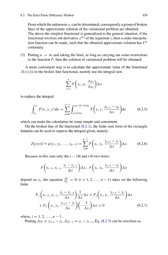
A more convenient way is to calculate the approximate value of the functional
J [y(x)] on the broken line functional, namely use the integral sum
n
i=1
F
x i , y i ,
y i
x i
x
to replace the integral
x 1
x 0
F(x, y, y
)dx =
n−1
k=0
x 0 +(k+1))x
x 0 +kx
F
x, y,
y k+1 − y k
x
dx
(8.2.5)
which can make the calculation be some simple and convenient.
On the broken line of the functional (8.2.1), the finite sum form of the rectangle
formula can be used to express the integral given, namely
J [y(x)] ≈ ϕ(y 1 , y 2 , . . . , y n−1 ) =
n−1
i=0
F
x i , y i ,
y i+1 − y i
x
x
(8.2.6)
Because in this sum only the i − 1th and i-th two terms
F
x i−1 , y i−1 ,
y i − y i−1
x
x, F
x i , y i ,
y i+1 − y i
x
x
depend on y i , the equation
∂ϕ
∂ y i
= 0 (i = 1, 2, . . . , n − 1) takes on the following
form
F y
x i−1 , y i−1 ,
y i − y i−1
x
1
x
x + F y
x i , y i ,
y i+1 − y i
x
x
+ F y
x i , y i ,
y i+1 − y i
x
−
1
x
x = 0
(8.2.7)
where, i = 1, 2, . . . , n − 1.
Putting y i = y i+1 − y i , y i−1 = y i − y i−1 , Eq. (8.2.7) can be rewritten as
459
From which the unknowns y i can be determined, consequently a group of broken
lines of the approximate solution of the variational problem are obtained.
The above the simplest functional is generalized to the general situation, if the
functional involves nth derivative y
(n) of the argument y, then n order interpolation function can be made, such that the obtained approximate solution has C
n
continuity.
(3) Putting n → ∞ and taking the limit, as long as carrying out some restrictions
to the function F, then the solution of variational problem will be obtained.
A more convenient way is to calculate the approximate value of the functional
J [y(x)] on the broken line functional, namely use the integral sum
n
i=1
F
x i , y i ,
y i
x i
x
to replace the integral
x 1
x 0
F(x, y, y
)dx =
n−1
k=0
x 0 +(k+1))x
x 0 +kx
F
x, y,
y k+1 − y k
x
dx
(8.2.5)
which can make the calculation be some simple and convenient.
On the broken line of the functional (8.2.1), the finite sum form of the rectangle
formula can be used to express the integral given, namely
J [y(x)] ≈ ϕ(y 1 , y 2 , . . . , y n−1 ) =
n−1
i=0
F
x i , y i ,
y i+1 − y i
x
x
(8.2.6)
Because in this sum only the i − 1th and i-th two terms
F
x i−1 , y i−1 ,
y i − y i−1
x
x, F
x i , y i ,
y i+1 − y i
x
x
depend on y i , the equation
∂ϕ
∂ y i
= 0 (i = 1, 2, . . . , n − 1) takes on the following
form
F y
x i−1 , y i−1 ,
y i − y i−1
x
1
x
x + F y
x i , y i ,
y i+1 − y i
x
x
+ F y
x i , y i ,
y i+1 − y i
x
−
1
x
x = 0
(8.2.7)
where, i = 1, 2, . . . , n − 1.
Putting y i = y i+1 − y i , y i−1 = y i − y i−1 , Eq. (8.2.7) can be rewritten as