

458
8 Direct Methods of Variational Problems
the boundary conditions are
y(x 0 ) = y 0 , y(x 1 ) = y 1
(8.2.2)
The general steps of approximate solution of variational problem to solve the
above functional are as follows:
(1) The interval [x 0 , x 1 ] is divided into n sections, where every section is called a
finite element, and every point of division is called the node. The lengths of the
units either may be equal, or may also not be equal. In each unit assuming that
the argument y is a function of the independent variable x, it can be written as
y(x) =
x i − x
x i − x i−1
y i−1 +
x − x i−1
x i − x i−1
y i (x i−1 ≤ x ≤ x i )
(8.2.3)
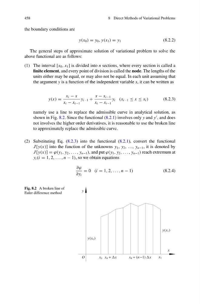
namely use a line to replace the admissible curve in analytical solution, as
shown in Fig. 8.2. Since the functional (8.2.1) involves only y and y
, and does
not involves the higher order derivatives, it is reasonable to use the broken line
to approximately replace the admissible curve.
(2) Substituting Eq. (8.2.3) into the functional (8.2.1), convert the functional
J [y(x)] into the function of the unknowns y 1 , y 2 , …, y n−1 , it is denoted by
J [y(x)] = ϕ(y 1 , y 2 , . . . , y n−1 ), and put ϕ(y 1 , y 2 , . . . , y n−1 ) reach extremum at
y i (i = 1, 2, . . . , n − 1), so we obtain equations
∂ϕ
∂ y i
= 0 (i = 1, 2, . . . , n − 1)
(8.2.4)
Fig. 8.2 A broken line of
Euler difference method
O
x 0 x 0 + x
x
x 0 (n −1)
x
x 1
y(x 0 )
y(x 1 )
y
8 Direct Methods of Variational Problems
the boundary conditions are
y(x 0 ) = y 0 , y(x 1 ) = y 1
(8.2.2)
The general steps of approximate solution of variational problem to solve the
above functional are as follows:
(1) The interval [x 0 , x 1 ] is divided into n sections, where every section is called a
finite element, and every point of division is called the node. The lengths of the
units either may be equal, or may also not be equal. In each unit assuming that
the argument y is a function of the independent variable x, it can be written as
y(x) =
x i − x
x i − x i−1
y i−1 +
x − x i−1
x i − x i−1
y i (x i−1 ≤ x ≤ x i )
(8.2.3)
namely use a line to replace the admissible curve in analytical solution, as
shown in Fig. 8.2. Since the functional (8.2.1) involves only y and y
, and does
not involves the higher order derivatives, it is reasonable to use the broken line
to approximately replace the admissible curve.
(2) Substituting Eq. (8.2.3) into the functional (8.2.1), convert the functional
J [y(x)] into the function of the unknowns y 1 , y 2 , …, y n−1 , it is denoted by
J [y(x)] = ϕ(y 1 , y 2 , . . . , y n−1 ), and put ϕ(y 1 , y 2 , . . . , y n−1 ) reach extremum at
y i (i = 1, 2, . . . , n − 1), so we obtain equations
∂ϕ
∂ y i
= 0 (i = 1, 2, . . . , n − 1)
(8.2.4)
Fig. 8.2 A broken line of
Euler difference method
O
x 0 x 0 + x
x
x 0 (n −1)
x
x 1
y(x 0 )
y(x 1 )
y