

8.1 Minimizing (Maximizing) Sequence
457
O
y
x
u
u = 0
u = A
u =
A
ln R ln
r
R
r = R
r = R
2
Γ
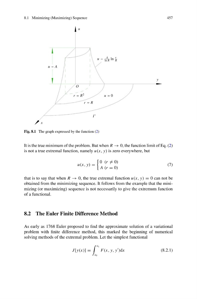
Fig. 8.1 The graph expressed by the function (2)
It is the true minimum of the problem. But when R → 0, the function limit of Eq. (2)
is not a true extremal function, namely u(x, y) is zero everywhere, but
u(x, y) =
0 (r = 0)
A (r = 0)
(7)
that is to say that when R → 0, the true extremal function u(x, y) = 0 can not be
obtained from the minimizing sequence. It follows from the example that the minimizing (or maximizing) sequence is not necessarily to give the extremum function
of a functional.
8.2 The Euler Finite Difference Method
As early as 1768 Euler proposed to find the approximate solution of a variational
problem with finite difference method, this marked the beginning of numerical
solving methods of the extremal problem. Let the simplest functional
J [y(x)] =
x 1
x 0
F(x, y, y
)dx
(8.2.1)
457
O
y
x
u
u = 0
u = A
u =
A
ln R ln
r
R
r = R
r = R
2
Γ
Fig. 8.1 The graph expressed by the function (2)
It is the true minimum of the problem. But when R → 0, the function limit of Eq. (2)
is not a true extremal function, namely u(x, y) is zero everywhere, but
u(x, y) =
0 (r = 0)
A (r = 0)
(7)
that is to say that when R → 0, the true extremal function u(x, y) = 0 can not be
obtained from the minimizing sequence. It follows from the example that the minimizing (or maximizing) sequence is not necessarily to give the extremum function
of a functional.
8.2 The Euler Finite Difference Method
As early as 1768 Euler proposed to find the approximate solution of a variational
problem with finite difference method, this marked the beginning of numerical
solving methods of the extremal problem. Let the simplest functional
J [y(x)] =
x 1
x 0
F(x, y, y
)dx
(8.2.1)