

414
7 Variational Principles
(T u, v) =
˚
V
[∇ · ( p∇u) + qu]vdV
=
˚
V
∇ · (v p∇u)dV −
˚
V
( p∇u · ∇v − quv)dV
=
S
v p
∂u
∂n
dS −
˚
V
( p∇u · ∇v − quv)dV
=
S
v p
∂u
∂n
dS −
S
up
∂v
∂n
dS +
˚
V
[u∇ · ( p∇v) + quv]dV
=
˚
V
u[∇ · ( p∇v) + qv]dV +
S
p
v
∂u
∂n
− u
∂v
∂n
dS
=
˚
V
u(T
∗ v)dV +
S
p
v
∂u
∂n
− u
∂v
∂n
dS
= (u, T
∗ v) +
S
p
v
∂u
∂n
− u
∂v
∂n
dS
(3)
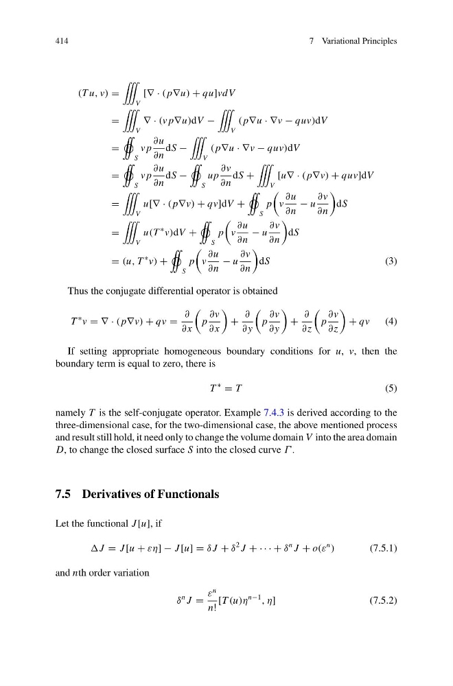
Thus the conjugate differential operator is obtained
T
∗ v = ∇ · ( p∇v) + qv =
∂
∂ x
p
∂v
∂ x
+
∂
∂ y
p
∂v
∂ y
+
∂
∂z
p
∂v
∂z
+ qv
(4)
If setting appropriate homogeneous boundary conditions for u, v, then the
boundary term is equal to zero, there is
T
∗
= T
(5)
namely T is the self-conjugate operator. Example 7.4.3 is derived according to the
three-dimensional case, for the two-dimensional case, the above mentioned process
and result still hold, it need only to change the volume domain V into the area domain
D, to change the closed surface S into the closed curve Γ .
7.5 Derivatives of Functionals
Let the functional J [u], if
J = J [u + εη] − J [u] = δ J + δ
2 J + · · · + δ
n J + o(ε
n
)
(7.5.1)
and nth order variation
δ
n J =
ε
n
n!
[T (u)η
n−1
, η]
(7.5.2)
7 Variational Principles
(T u, v) =
˚
V
[∇ · ( p∇u) + qu]vdV
=
˚
V
∇ · (v p∇u)dV −
˚
V
( p∇u · ∇v − quv)dV
=
S
v p
∂u
∂n
dS −
˚
V
( p∇u · ∇v − quv)dV
=
S
v p
∂u
∂n
dS −
S
up
∂v
∂n
dS +
˚
V
[u∇ · ( p∇v) + quv]dV
=
˚
V
u[∇ · ( p∇v) + qv]dV +
S
p
v
∂u
∂n
− u
∂v
∂n
dS
=
˚
V
u(T
∗ v)dV +
S
p
v
∂u
∂n
− u
∂v
∂n
dS
= (u, T
∗ v) +
S
p
v
∂u
∂n
− u
∂v
∂n
dS
(3)
Thus the conjugate differential operator is obtained
T
∗ v = ∇ · ( p∇v) + qv =
∂
∂ x
p
∂v
∂ x
+
∂
∂ y
p
∂v
∂ y
+
∂
∂z
p
∂v
∂z
+ qv
(4)
If setting appropriate homogeneous boundary conditions for u, v, then the
boundary term is equal to zero, there is
T
∗
= T
(5)
namely T is the self-conjugate operator. Example 7.4.3 is derived according to the
three-dimensional case, for the two-dimensional case, the above mentioned process
and result still hold, it need only to change the volume domain V into the area domain
D, to change the closed surface S into the closed curve Γ .
7.5 Derivatives of Functionals
Let the functional J [u], if
J = J [u + εη] − J [u] = δ J + δ
2 J + · · · + δ
n J + o(ε
n
)
(7.5.1)
and nth order variation
δ
n J =
ε
n
n!
[T (u)η
n−1
, η]
(7.5.2)