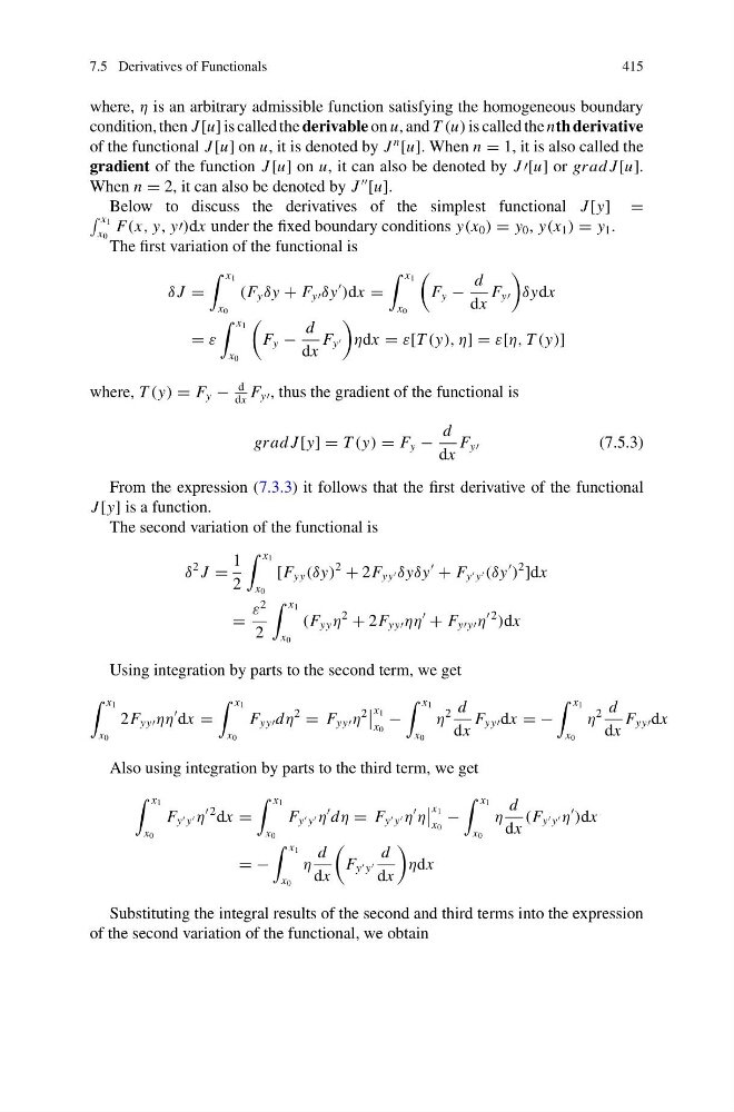
7.5 Derivatives of Functionals
415
where, η is an arbitrary admissible function satisfying the homogeneous boundary
condition, then J [u] is called the derivable on u, and T (u) is called the nth derivative
of the functional J [u] on u, it is denoted by J
n
[u]. When n = 1, it is also called the
gradient of the function J [u] on u, it can also be denoted by J [u] or grad J [u].
When n = 2, it can also be denoted by J
[u].
Below to discuss the derivatives of the simplest functional J [y] =
x 1
x 0
F(x, y, y)dx under the fixed boundary conditions y(x 0 ) = y 0 , y(x 1 ) = y 1 .
The first variation of the functional is
δ J =
x 1
x 0
(F y δy + F y δy
)dx =
x 1
x 0
F y −
d
dx
F y
δydx
= ε
x 1
x 0
F y −
d
dx
F y
ηdx = ε[T (y), η] = ε[η, T (y)]
where, T (y) = F y −
d
dx
F y , thus the gradient of the functional is
grad J [y] = T (y) = F y −
d
dx
F y
(7.5.3)
From the expression (7.3.3) it follows that the first derivative of the functional
J [y] is a function.
The second variation of the functional is
δ
2 J =
1
2
x 1
x 0
[F yy (δy)
2
+ 2F yy δyδy
+ F y y (δy
)
2
]dx
=
ε
2
2
x 1
x 0
(F yy η
2
+ 2F yy ηη
+ F yy η
2
)dx
Using integration by parts to the second term, we get
x 1
x 0
2F yy ηη
dx =
x 1
x 0
F yy dη
2
= F yy η
2
x 1
x 0
−
x 1
x 0
η
2 d
dx
F yy dx = −
x 1
x 0
η
2 d
dx
F yy dx
Also using integration by parts to the third term, we get
x 1
x 0
F y y η
2 dx =
x 1
x 0
F y y η
dη = F y y η
η
x 1
x 0
−
x 1
x 0
η
d
dx
(F y y η
)dx
= −
x 1
x 0
η
d
dx
F y y
d
dx
ηdx
Substituting the integral results of the second and third terms into the expression
of the second variation of the functional, we obtain