

6.3 Extrema of Functionals with Variable Boundaries and Parametric Forms
379
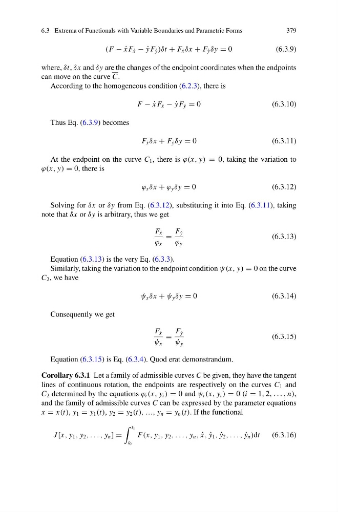
(F − ˙
x F ˙
x − ˙
y F ˙
y )δt + F ˙
x δx + F ˙
y δy = 0
(6.3.9)
where, δt, δx and δy are the changes of the endpoint coordinates when the endpoints
can move on the curve C.
According to the homogeneous condition (6.2.3), there is
F − ˙
x F ˙
x − ˙
y F ˙
y = 0
(6.3.10)
Thus Eq. (6.3.9) becomes
F ˙
x δx + F ˙
y δy = 0
(6.3.11)
At the endpoint on the curve C 1 , there is ϕ(x, y) = 0, taking the variation to
ϕ(x, y) = 0, there is
ϕ x δx + ϕ y δy = 0
(6.3.12)
Solving for δx or δy from Eq. (6.3.12), substituting it into Eq. (6.3.11), taking
note that δx or δy is arbitrary, thus we get
F ˙
x
ϕ x
=
F ˙
y
ϕ y
(6.3.13)
Equation (6.3.13) is the very Eq. (6.3.3).
Similarly, taking the variation to the endpoint condition ψ(x, y) = 0 on the curve
C 2 , we have
ψ x δx + ψ y δy = 0
(6.3.14)
Consequently we get
F ˙
x
ψ x
=
F ˙
y
ψ y
(6.3.15)
Equation (6.3.15) is Eq. (6.3.4). Quod erat demonstrandum.
Corollary 6.3.1 Let a family of admissible curves C be given, they have the tangent
lines of continuous rotation, the endpoints are respectively on the curves C 1 and
C 2 determined by the equations ϕ i (x, y i ) = 0 and ψ i (x, y i ) = 0 (i = 1, 2, . . . , n),
and the family of admissible curves C can be expressed by the parameter equations
x = x(t), y 1 = y 1 (t), y 2 = y 2 (t), …, y n = y n (t). If the functional
J [x, y 1 , y 2 , . . . , y n ] =
t 1
t 0
F(x, y 1 , y 2 , . . . , y n , ˙
x, ˙
y 1 , ˙
y 2 , . . . , ˙
y n )dt
(6.3.16)
379
(F − ˙
x F ˙
x − ˙
y F ˙
y )δt + F ˙
x δx + F ˙
y δy = 0
(6.3.9)
where, δt, δx and δy are the changes of the endpoint coordinates when the endpoints
can move on the curve C.
According to the homogeneous condition (6.2.3), there is
F − ˙
x F ˙
x − ˙
y F ˙
y = 0
(6.3.10)
Thus Eq. (6.3.9) becomes
F ˙
x δx + F ˙
y δy = 0
(6.3.11)
At the endpoint on the curve C 1 , there is ϕ(x, y) = 0, taking the variation to
ϕ(x, y) = 0, there is
ϕ x δx + ϕ y δy = 0
(6.3.12)
Solving for δx or δy from Eq. (6.3.12), substituting it into Eq. (6.3.11), taking
note that δx or δy is arbitrary, thus we get
F ˙
x
ϕ x
=
F ˙
y
ϕ y
(6.3.13)
Equation (6.3.13) is the very Eq. (6.3.3).
Similarly, taking the variation to the endpoint condition ψ(x, y) = 0 on the curve
C 2 , we have
ψ x δx + ψ y δy = 0
(6.3.14)
Consequently we get
F ˙
x
ψ x
=
F ˙
y
ψ y
(6.3.15)
Equation (6.3.15) is Eq. (6.3.4). Quod erat demonstrandum.
Corollary 6.3.1 Let a family of admissible curves C be given, they have the tangent
lines of continuous rotation, the endpoints are respectively on the curves C 1 and
C 2 determined by the equations ϕ i (x, y i ) = 0 and ψ i (x, y i ) = 0 (i = 1, 2, . . . , n),
and the family of admissible curves C can be expressed by the parameter equations
x = x(t), y 1 = y 1 (t), y 2 = y 2 (t), …, y n = y n (t). If the functional
J [x, y 1 , y 2 , . . . , y n ] =
t 1
t 0
F(x, y 1 , y 2 , . . . , y n , ˙
x, ˙
y 1 , ˙
y 2 , . . . , ˙
y n )dt
(6.3.16)