

380
6 Variational Problems in Parametric Forms
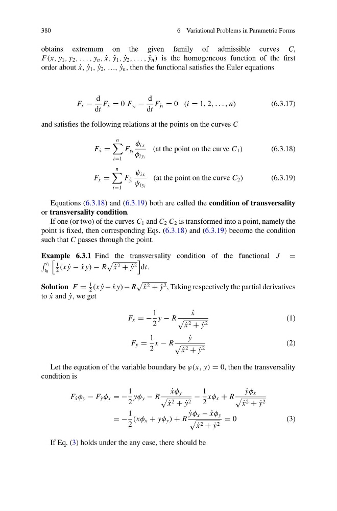
obtains extremum on the given family of admissible curves C,
F(x, y 1 , y 2 , . . . , y n , ˙
x, ˙
y 1 , ˙
y 2 , . . . , ˙
y n ) is the homogeneous function of the first
order about ˙
x, ˙
y 1 , ˙
y 2 , …, ˙
y n , then the functional satisfies the Euler equations
F x −
d
dt
F ˙
x = 0 F y i −
d
dt
F ˙
y i = 0 (i = 1, 2, . . . , n)
(6.3.17)
and satisfies the following relations at the points on the curves C
F ˙
x =
n
i=1
F ˙
y i
φ i x
φ iy i
(at the point on the curve C 1 )
(6.3.18)
F ˙
x =
n
i=1
F ˙
y i
ψ i x
ψ iy i
(at the point on the curve C 2 )
(6.3.19)
Equations (6.3.18) and (6.3.19) both are called the condition of transversality
or transversality condition.
If one (or two) of the curves C 1 and C 2 C 2 is transformed into a point, namely the
point is fixed, then corresponding Eqs. (6.3.18) and (6.3.19) become the condition
such that C passes through the point.
Example 6.3.1 Find the transversality condition of the functional J =
t 1
t 0
1
2
(x ˙
y − ˙
x y) − R
˙
x 2 + ˙
y 2
dt.
Solution F =
1
2
(x ˙
y − ˙
x y) − R
˙
x 2 + ˙
y 2 , Taking respectively the partial derivatives
to ˙
x and ˙
y, we get
F ˙
x = −
1
2
y − R
˙
x
˙
x 2 + ˙
y 2
(1)
F ˙
y =
1
2
x − R
˙
y
˙
x 2 + ˙
y 2
(2)
Let the equation of the variable boundary be ϕ(x, y) = 0, then the transversality
condition is
F ˙
x φ y − F ˙
y φ x = −
1
2
yφ y − R
˙
xφ y
˙
x 2 + ˙
y 2
−
1
2
xφ x + R
˙
yφ x
˙
x 2 + ˙
y 2
= −
1
2
(xφ x + yφ y ) + R
˙
yφ x − ˙
xφ y
˙
x 2 + ˙
y 2
= 0
( 3 )
If Eq. (3) holds under the any case, there should be
6 Variational Problems in Parametric Forms
obtains extremum on the given family of admissible curves C,
F(x, y 1 , y 2 , . . . , y n , ˙
x, ˙
y 1 , ˙
y 2 , . . . , ˙
y n ) is the homogeneous function of the first
order about ˙
x, ˙
y 1 , ˙
y 2 , …, ˙
y n , then the functional satisfies the Euler equations
F x −
d
dt
F ˙
x = 0 F y i −
d
dt
F ˙
y i = 0 (i = 1, 2, . . . , n)
(6.3.17)
and satisfies the following relations at the points on the curves C
F ˙
x =
n
i=1
F ˙
y i
φ i x
φ iy i
(at the point on the curve C 1 )
(6.3.18)
F ˙
x =
n
i=1
F ˙
y i
ψ i x
ψ iy i
(at the point on the curve C 2 )
(6.3.19)
Equations (6.3.18) and (6.3.19) both are called the condition of transversality
or transversality condition.
If one (or two) of the curves C 1 and C 2 C 2 is transformed into a point, namely the
point is fixed, then corresponding Eqs. (6.3.18) and (6.3.19) become the condition
such that C passes through the point.
Example 6.3.1 Find the transversality condition of the functional J =
t 1
t 0
1
2
(x ˙
y − ˙
x y) − R
˙
x 2 + ˙
y 2
dt.
Solution F =
1
2
(x ˙
y − ˙
x y) − R
˙
x 2 + ˙
y 2 , Taking respectively the partial derivatives
to ˙
x and ˙
y, we get
F ˙
x = −
1
2
y − R
˙
x
˙
x 2 + ˙
y 2
(1)
F ˙
y =
1
2
x − R
˙
y
˙
x 2 + ˙
y 2
(2)
Let the equation of the variable boundary be ϕ(x, y) = 0, then the transversality
condition is
F ˙
x φ y − F ˙
y φ x = −
1
2
yφ y − R
˙
xφ y
˙
x 2 + ˙
y 2
−
1
2
xφ x + R
˙
yφ x
˙
x 2 + ˙
y 2
= −
1
2
(xφ x + yφ y ) + R
˙
yφ x − ˙
xφ y
˙
x 2 + ˙
y 2
= 0
( 3 )
If Eq. (3) holds under the any case, there should be