

378
6 Variational Problems in Parametric Forms
F ˙
x
φ x
=
F ˙
y
φ y
(at the endpoint on the curve C 1 )
(6.3.3)
F ˙
x
ψ x
=
F ˙
y
ψ y
(at the endpoint on the curve C 2 )
(6.3.4)
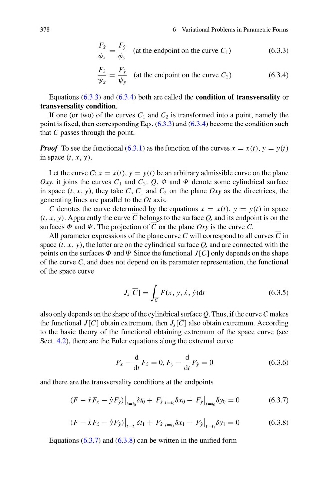
Equations (6.3.3) and (6.3.4) both are called the condition of transversality or
transversality condition.
If one (or two) of the curves C 1 and C 2 is transformed into a point, namely the
point is fixed, then corresponding Eqs. (6.3.3) and (6.3.4) become the condition such
that C passes through the point.
Proof To see the functional (6.3.1) as the function of the curves x = x(t), y = y(t)
in space (t, x, y).
Let the curve C: x = x(t), y = y(t) be an arbitrary admissible curve on the plane
Oxy, it joins the curves C 1 and C 2 . Q, Φ and Ψ denote some cylindrical surface
in space (t, x, y), they take C, C 1 and C 2 on the plane Oxy as the directrices, the
generating lines are parallel to the Ot axis.
C denotes the curve determined by the equations x = x(t), y = y(t) in space
(t, x, y). Apparently the curve C belongs to the surface Q, and its endpoint is on the
surfaces Φ and Ψ . The projection of C on the plane Oxy is the curve C.
All parameter expressions of the plane curve C will correspond to all curves C in
space (t, x, y), the latter are on the cylindrical surface Q, and are connected with the
points on the surfaces Φ and Ψ Since the functional J [C] only depends on the shape
of the curve C, and does not depend on its parameter representation, the functional
of the space curve
J s [C] =
C
F(x, y, ˙
x, ˙
y)dt
(6.3.5)
also only depends on the shape of the cylindrical surface Q. Thus, if the curve C makes
the functional J [C] obtain extremum, then J s [C] also obtain extremum. According
to the basic theory of the functional obtaining extremum of the space curve (see
Sect. 4.2), there are the Euler equations along the extremal curve
F x −
d
dt
F ˙
x = 0, F y −
d
dt
F ˙
y = 0
(6.3.6)
and there are the transversality conditions at the endpoints
(F − ˙
x F ˙
x − ˙
y F ˙
y )
t=t 0
δt 0 + F ˙
x | t=t 0 δx 0 + F ˙
y
t=t 0
δy 0 = 0
(6.3.7)
(F − ˙
x F ˙
x − ˙
y F ˙
y )
t=t 1
δt 1 + F ˙
x | t=t 1 δx 1 + F ˙
y
t=t 1
δy 1 = 0
(6.3.8)
Equations (6.3.7) and (6.3.8) can be written in the unified form
6 Variational Problems in Parametric Forms
F ˙
x
φ x
=
F ˙
y
φ y
(at the endpoint on the curve C 1 )
(6.3.3)
F ˙
x
ψ x
=
F ˙
y
ψ y
(at the endpoint on the curve C 2 )
(6.3.4)
Equations (6.3.3) and (6.3.4) both are called the condition of transversality or
transversality condition.
If one (or two) of the curves C 1 and C 2 is transformed into a point, namely the
point is fixed, then corresponding Eqs. (6.3.3) and (6.3.4) become the condition such
that C passes through the point.
Proof To see the functional (6.3.1) as the function of the curves x = x(t), y = y(t)
in space (t, x, y).
Let the curve C: x = x(t), y = y(t) be an arbitrary admissible curve on the plane
Oxy, it joins the curves C 1 and C 2 . Q, Φ and Ψ denote some cylindrical surface
in space (t, x, y), they take C, C 1 and C 2 on the plane Oxy as the directrices, the
generating lines are parallel to the Ot axis.
C denotes the curve determined by the equations x = x(t), y = y(t) in space
(t, x, y). Apparently the curve C belongs to the surface Q, and its endpoint is on the
surfaces Φ and Ψ . The projection of C on the plane Oxy is the curve C.
All parameter expressions of the plane curve C will correspond to all curves C in
space (t, x, y), the latter are on the cylindrical surface Q, and are connected with the
points on the surfaces Φ and Ψ Since the functional J [C] only depends on the shape
of the curve C, and does not depend on its parameter representation, the functional
of the space curve
J s [C] =
C
F(x, y, ˙
x, ˙
y)dt
(6.3.5)
also only depends on the shape of the cylindrical surface Q. Thus, if the curve C makes
the functional J [C] obtain extremum, then J s [C] also obtain extremum. According
to the basic theory of the functional obtaining extremum of the space curve (see
Sect. 4.2), there are the Euler equations along the extremal curve
F x −
d
dt
F ˙
x = 0, F y −
d
dt
F ˙
y = 0
(6.3.6)
and there are the transversality conditions at the endpoints
(F − ˙
x F ˙
x − ˙
y F ˙
y )
t=t 0
δt 0 + F ˙
x | t=t 0 δx 0 + F ˙
y
t=t 0
δy 0 = 0
(6.3.7)
(F − ˙
x F ˙
x − ˙
y F ˙
y )
t=t 1
δt 1 + F ˙
x | t=t 1 δx 1 + F ˙
y
t=t 1
δy 1 = 0
(6.3.8)
Equations (6.3.7) and (6.3.8) can be written in the unified form