

5.1 Variational Problems with Holonomic Constraints
323
⎧
⎪ ⎪ ⎪ ⎪ ⎨
⎪ ⎪ ⎪ ⎪ ⎩
λϕ y −
d
dx
y
1 + y 2 + z 2
= 0
λϕ z −
d
dx
z
1 + y 2 + z 2
= 0
ϕ(x, y, z) = 0
(5.3)
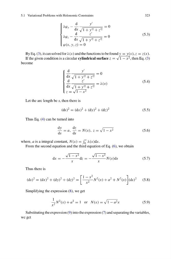
By Eq. (3), it can solved for λ(x) and the functions to be found y = y(x), z = z(x).
If the given condition is a circular cylindrical surface z =
√
1 − x 2 , then Eq. (3)
become
⎧
⎪ ⎪ ⎪ ⎪ ⎨
⎪ ⎪ ⎪ ⎪ ⎩
d
dx
y
1 + y 2 + z 2
= 0
d
dx
z
1 + y 2 + z 2
= λ(x)
z =
√
1 − x 2
(5.4)
Let the arc length be s, then there is
(ds)
2
= (dx)
2
+ (dy)
2
+ (dz)
2
(5.5)
Thus Eq. (4) can be turned into
dy
ds
= a,
dz
ds
= N (x), z =
1 − x 2
(5.6)
where, a is a integral constant, N (x) =
x
0 λ(x)dx.
From the second equation and the third equation of Eq. (6), we obtain
dx = −
√
1 − x 2
x
dz = −
√
1 − x 2
x
N (x)ds
(5.7)
Thus there is
(ds)
2
= (dx)
2
+ (dy)
2
+ (dz)
2
=
1 − x
2
x 2 N
2
(x) + a
2
+ N
2
(x)
(ds)
2
(5.8)
Simplifying the expression (8), we get
1
x 2 N
2
(x) + a
2
= 1 or N (x) =
1 − a 2 x
(5.9)
Substituting the expression (9) into the expression (7) and separating the variables,
we get
323
⎧
⎪ ⎪ ⎪ ⎪ ⎨
⎪ ⎪ ⎪ ⎪ ⎩
λϕ y −
d
dx
y
1 + y 2 + z 2
= 0
λϕ z −
d
dx
z
1 + y 2 + z 2
= 0
ϕ(x, y, z) = 0
(5.3)
By Eq. (3), it can solved for λ(x) and the functions to be found y = y(x), z = z(x).
If the given condition is a circular cylindrical surface z =
√
1 − x 2 , then Eq. (3)
become
⎧
⎪ ⎪ ⎪ ⎪ ⎨
⎪ ⎪ ⎪ ⎪ ⎩
d
dx
y
1 + y 2 + z 2
= 0
d
dx
z
1 + y 2 + z 2
= λ(x)
z =
√
1 − x 2
(5.4)
Let the arc length be s, then there is
(ds)
2
= (dx)
2
+ (dy)
2
+ (dz)
2
(5.5)
Thus Eq. (4) can be turned into
dy
ds
= a,
dz
ds
= N (x), z =
1 − x 2
(5.6)
where, a is a integral constant, N (x) =
x
0 λ(x)dx.
From the second equation and the third equation of Eq. (6), we obtain
dx = −
√
1 − x 2
x
dz = −
√
1 − x 2
x
N (x)ds
(5.7)
Thus there is
(ds)
2
= (dx)
2
+ (dy)
2
+ (dz)
2
=
1 − x
2
x 2 N
2
(x) + a
2
+ N
2
(x)
(ds)
2
(5.8)
Simplifying the expression (8), we get
1
x 2 N
2
(x) + a
2
= 1 or N (x) =
1 − a 2 x
(5.9)
Substituting the expression (9) into the expression (7) and separating the variables,
we get