

4.5 Extremal Curves with Cuspidal Points
301
O
x
y
A
B
C
n 1 (x, y)
n 2 (x, y)
y = ϕ(x)
α
β 1
β 2
α− β 1
α − β 2
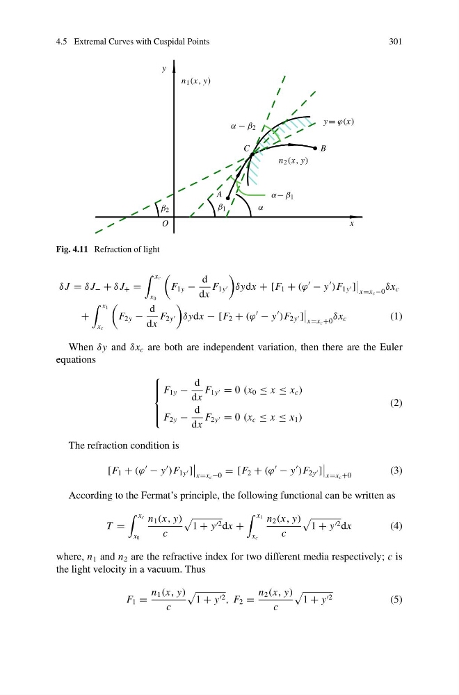
Fig. 4.11 Refraction of light
δ J = δ J − + δ J + =
x c
x 0
F 1y −
d
dx
F 1y
δydx + [F 1 + (ϕ
− y
)F 1y ]
x=x c −0
δx c
+
x 1
x c
F 2y −
d
dx
F 2y
δydx − [F 2 + (ϕ
− y
)F 2y ]
x=x c +0
δx c
(1)
When δy and δx c are both are independent variation, then there are the Euler
equations
⎧
⎪ ⎪ ⎨
⎪ ⎪ ⎩
F 1y −
d
dx
F 1y = 0 (x 0 ≤ x ≤ x c )
F 2y −
d
dx
F 2y = 0 (x c ≤ x ≤ x 1 )
(2)
The refraction condition is
[F 1 + (ϕ
− y
)F 1y ]
x=x c −0
= [F 2 + (ϕ
− y
)F 2y ]
x=x c +0
(3)
According to the Fermat’s principle, the following functional can be written as
T =
x c
x 0
n 1 (x, y)
c
1 + y dx +
x 1
x c
n 2 (x, y)
c
1 + y dx
(4)
where, n 1 and n 2 are the refractive index for two different media respectively; c is
the light velocity in a vacuum. Thus
F 1 =
n 1 (x, y)
c
1 + y , F 2 =
n 2 (x, y)
c
1 + y
(5)
301
O
x
y
A
B
C
n 1 (x, y)
n 2 (x, y)
y = ϕ(x)
α
β 1
β 2
α− β 1
α − β 2
Fig. 4.11 Refraction of light
δ J = δ J − + δ J + =
x c
x 0
F 1y −
d
dx
F 1y
δydx + [F 1 + (ϕ
− y
)F 1y ]
x=x c −0
δx c
+
x 1
x c
F 2y −
d
dx
F 2y
δydx − [F 2 + (ϕ
− y
)F 2y ]
x=x c +0
δx c
(1)
When δy and δx c are both are independent variation, then there are the Euler
equations
⎧
⎪ ⎪ ⎨
⎪ ⎪ ⎩
F 1y −
d
dx
F 1y = 0 (x 0 ≤ x ≤ x c )
F 2y −
d
dx
F 2y = 0 (x c ≤ x ≤ x 1 )
(2)
The refraction condition is
[F 1 + (ϕ
− y
)F 1y ]
x=x c −0
= [F 2 + (ϕ
− y
)F 2y ]
x=x c +0
(3)
According to the Fermat’s principle, the following functional can be written as
T =
x c
x 0
n 1 (x, y)
c
1 + y dx +
x 1
x c
n 2 (x, y)
c
1 + y dx
(4)
where, n 1 and n 2 are the refractive index for two different media respectively; c is
the light velocity in a vacuum. Thus
F 1 =
n 1 (x, y)
c
1 + y , F 2 =
n 2 (x, y)
c
1 + y
(5)