

298
4 Problems with Variable Boundaries
solutions of y
x=x c −0
= y
x=x c +0
y
(x c − 0) = 0, y
(x c + 0) = 1
( 2 )
or
y
(x c − 0) = 1, y
(x c + 0) = 0
( 3 )
Hence no matter on which side of x = x c the extremal curve is a straight line. If
the slope is zero at the broken point, then the straight runs parallel to the x axis, if
the slope is 1 at the broken point, then the straight line is at an angle 45° from the x
axis. This shows that the extremal curve only consists of the family of straight lines
y = c 1 and y = x + c 2 , as shown in Fig. 4.8.
Now through two examples to discuss two kinds of special cuspidal point cases.
Example 4.5.2 The reflection problem of the extremal curve. This problem is a
generalization of the problem of light reflection. Let the function y = y(x) make
the functional J [y] =
x 1
x 0
F(x, y, y
)dx attain extremum, and y = y(x) passes
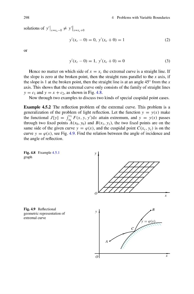
through two fixed points A(x 0 , y 0 ) and B(x 1 , y 1 ), the two fixed points are on the
same side of the given curve y = ϕ(x), and the cuspidal point C(x c , y c ) is on the
curve y = ϕ(x), see Fig. 4.9. Find the relation between the angle of incidence and
the angle of reflection.
Fig. 4.8 Example 4.5.1
graph
O
x
y
Fig. 4.9 Reflectional
geometric representation of
extremal curve
O
x
y
A
B
C
y = ϕ(x)
4 Problems with Variable Boundaries
solutions of y
x=x c −0
= y
x=x c +0
y
(x c − 0) = 0, y
(x c + 0) = 1
( 2 )
or
y
(x c − 0) = 1, y
(x c + 0) = 0
( 3 )
Hence no matter on which side of x = x c the extremal curve is a straight line. If
the slope is zero at the broken point, then the straight runs parallel to the x axis, if
the slope is 1 at the broken point, then the straight line is at an angle 45° from the x
axis. This shows that the extremal curve only consists of the family of straight lines
y = c 1 and y = x + c 2 , as shown in Fig. 4.8.
Now through two examples to discuss two kinds of special cuspidal point cases.
Example 4.5.2 The reflection problem of the extremal curve. This problem is a
generalization of the problem of light reflection. Let the function y = y(x) make
the functional J [y] =
x 1
x 0
F(x, y, y
)dx attain extremum, and y = y(x) passes
through two fixed points A(x 0 , y 0 ) and B(x 1 , y 1 ), the two fixed points are on the
same side of the given curve y = ϕ(x), and the cuspidal point C(x c , y c ) is on the
curve y = ϕ(x), see Fig. 4.9. Find the relation between the angle of incidence and
the angle of reflection.
Fig. 4.8 Example 4.5.1
graph
O
x
y
Fig. 4.9 Reflectional
geometric representation of
extremal curve
O
x
y
A
B
C
y = ϕ(x)