

280
4 Problems with Variable Boundaries
δy
( j)
= ψ
j (x)δx
(4.3.29)
Since x and y are at the right endpoint, x = x 1 , y = y 1 , thus the relation (4.3.28)
and relation (4.3.29) can be written as
δy 1 = ϕ
(x 1 )δx 1
(4.3.30)
δy
( j)
1 = ψ
j (x 1 )δx 1
(4.3.31)
Substituting the relation (4.3.30) and relation (4.3.31) into the formula (4.3.25),
and according to the arbitrariness of δx 1 , the Eq. (4.3.27) can be obtained certainly.
Quod erat demonstrandum.
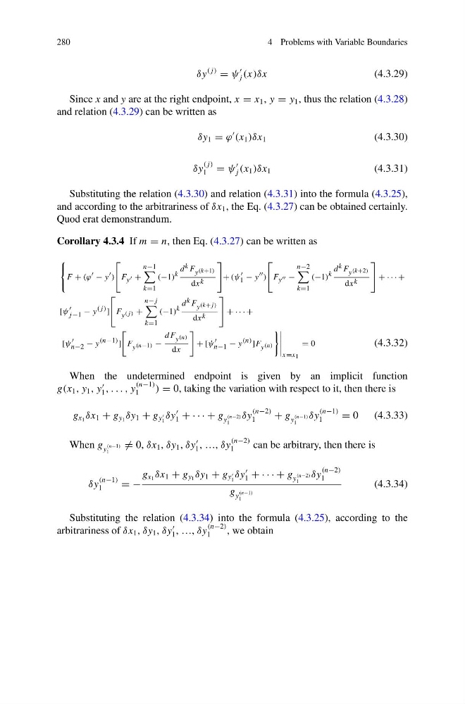
Corollary 4.3.4 If m = n, then Eq. (4.3.27) can be written as
⎧
⎨
⎩
F + (ϕ − y )
⎡
⎣ F y +
n−1
k=1
(−1) k
d k F y (k+1)
dx k
⎤
⎦ + (ψ
1 − y )
⎡
⎣ F y −
n−2
k=1
(−1) k
d k F y (k+2)
dx k
⎤
⎦ + · · · +
[ψ
j−1 − y ( j) ]
⎡
⎣ F y ( j) +
n− j
k=1
(−1) k
d k F y (k+ j)
dx k
⎤
⎦ + · · · +
[ψ
n−2 − y (n−1) ]
F y (n−1) −
d F y (n)
dx
+ [ψ
n−1 − y (n) ]F y (n)
x=x 1
= 0
(4.3.32)
When the undetermined endpoint is given by an implicit function
g(x 1 , y 1 , y
1 , . . . , y
(n−1)
1
) = 0, taking the variation with respect to it, then there is
g x 1 δx 1 + g y 1 δy 1 + g y
1
δy
1 + · · · + g y
(n−2)
1
δy
(n−2)
1
+ g y
(n−1)
1
δy
(n−1)
1
= 0
(4.3.33)
When g y
(n−1)
1
= 0, δx 1 , δy 1 , δy
1 , …, δy
(n−2)
1
can be arbitrary, then there is
δy
(n−1)
1
= −
g x 1 δx 1 + g y 1 δy 1 + g y
1
δy
1 + · · · + g y
(n−2)
1
δy
(n−2)
1
g y
(n−1)
1
(4.3.34)
Substituting the relation (4.3.34) into the formula (4.3.25), according to the
arbitrariness of δx 1 , δy 1 , δy
1 , …, δy
(n−2)
1
, we obtain
4 Problems with Variable Boundaries
δy
( j)
= ψ
j (x)δx
(4.3.29)
Since x and y are at the right endpoint, x = x 1 , y = y 1 , thus the relation (4.3.28)
and relation (4.3.29) can be written as
δy 1 = ϕ
(x 1 )δx 1
(4.3.30)
δy
( j)
1 = ψ
j (x 1 )δx 1
(4.3.31)
Substituting the relation (4.3.30) and relation (4.3.31) into the formula (4.3.25),
and according to the arbitrariness of δx 1 , the Eq. (4.3.27) can be obtained certainly.
Quod erat demonstrandum.
Corollary 4.3.4 If m = n, then Eq. (4.3.27) can be written as
⎧
⎨
⎩
F + (ϕ − y )
⎡
⎣ F y +
n−1
k=1
(−1) k
d k F y (k+1)
dx k
⎤
⎦ + (ψ
1 − y )
⎡
⎣ F y −
n−2
k=1
(−1) k
d k F y (k+2)
dx k
⎤
⎦ + · · · +
[ψ
j−1 − y ( j) ]
⎡
⎣ F y ( j) +
n− j
k=1
(−1) k
d k F y (k+ j)
dx k
⎤
⎦ + · · · +
[ψ
n−2 − y (n−1) ]
F y (n−1) −
d F y (n)
dx
+ [ψ
n−1 − y (n) ]F y (n)
x=x 1
= 0
(4.3.32)
When the undetermined endpoint is given by an implicit function
g(x 1 , y 1 , y
1 , . . . , y
(n−1)
1
) = 0, taking the variation with respect to it, then there is
g x 1 δx 1 + g y 1 δy 1 + g y
1
δy
1 + · · · + g y
(n−2)
1
δy
(n−2)
1
+ g y
(n−1)
1
δy
(n−1)
1
= 0
(4.3.33)
When g y
(n−1)
1
= 0, δx 1 , δy 1 , δy
1 , …, δy
(n−2)
1
can be arbitrary, then there is
δy
(n−1)
1
= −
g x 1 δx 1 + g y 1 δy 1 + g y
1
δy
1 + · · · + g y
(n−2)
1
δy
(n−2)
1
g y
(n−1)
1
(4.3.34)
Substituting the relation (4.3.34) into the formula (4.3.25), according to the
arbitrariness of δx 1 , δy 1 , δy
1 , …, δy
(n−2)
1
, we obtain