

4.3 Variational Problems of Functionals with Higher Order Derivatives
279
Equation (4.3.26) is the natural boundary conditions required by the functional
obtaining extremmum under the condition of δx 1 = 0.
There are n natural boundary conditions in Eq. (4.3.26), with n boundary conditions at the fixed endpoint, there are 2n boundary conditions in all, x 1 is known at
this moment, integrating the Euler Eq. (4.3.16), then the 2n undetermined constants
in the extremal function y = y(x, c 1 , c 2 , . . . , c i , . . . , c 2n , x 1 ) can be determined.
Based on the above analysis, a theorem of the variational problem of the functional
depending on an argument, an unknown function and its from first to n-th derivative
can be obtained, it can be stated as follows.
Theorem 4.3.2 Let the left endpoint of the extremal function y = y(x) of the
functional (4.3.15) be fixed, while another endpoint is undetermined on the straght
line x = x 1 , then the undetermined endpoint must satisfy the natural boundary
condition (4.3.26).
If the left endpoint of the extremal functin y = y(x) is fixed, while the right
endpoint is undetermined on the known curve y = ψ(x), then the variation δx 1 has
to do with δy 1 , δy
1 , …, δy
(n−1)
1
. Correspondently, there is the following theorem:
Theorem 4.3.3 Let the left endpoint of the extremal function y = y(x) of the
functional (4.3.15) be fixed, while the right endpoint is undetermined on the known
curve y = ϕ(x), and at the right endpoint the j-th derivative of the extremal function
y = y(x) is another known function y
( j)
= ψ j (x) of the right endpoint x 1 , where
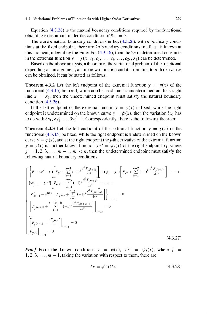
j = 1, 2, 3, . . . , m − 1, m < n, then the undetermined endpoint must satisfy the
following natural boundary conditions
⎧
⎪ ⎪ ⎪ ⎪ ⎪ ⎪ ⎪ ⎪ ⎪ ⎪ ⎪ ⎪ ⎪ ⎪ ⎪ ⎪ ⎪ ⎪ ⎪ ⎪ ⎪ ⎪ ⎪ ⎪ ⎨
⎪ ⎪ ⎪ ⎪ ⎪ ⎪ ⎪ ⎪ ⎪ ⎪ ⎪ ⎪ ⎪ ⎪ ⎪ ⎪ ⎪ ⎪ ⎪ ⎪ ⎪ ⎪ ⎪ ⎪ ⎩
F + (ϕ − y )
F y +
n−1
k=1
(−1) k
d k F y (k+1)
dx k
+ (ψ
1 − y )
F y +
n−2
k=1
(−1) k
d k F y (k+2)
dx k
+ · · · +
[ψ
j−1 − y ( j) ]
F y ( j) +
n− j
k=1
(−1) k
d k F y (k+ j)
dx k
+ · · · +
[ψ
m−1 − y (m) ]
F y (m) +
n−m
k=1
(−1) k
d k F y (k+m)
dx k
x=x 1
= 0
F y (m+1) +
n−(m+1)
k=1
(−1) k
d k F y (k+m+1)
dx k
x=x 1
= 0
. . .
F y (n−1) −
d F y (n)
dx
x=x 1
= 0
F y (n)
x=x 1
= 0
(4.3.27)
Proof From the known conditions y = ϕ(x), y
( j)
= ψ j (x), where j =
1, 2, 3, . . . , m − 1, taking the variation with respect to them, there are
δy = ϕ
(x)δx
(4.3.28)
279
Equation (4.3.26) is the natural boundary conditions required by the functional
obtaining extremmum under the condition of δx 1 = 0.
There are n natural boundary conditions in Eq. (4.3.26), with n boundary conditions at the fixed endpoint, there are 2n boundary conditions in all, x 1 is known at
this moment, integrating the Euler Eq. (4.3.16), then the 2n undetermined constants
in the extremal function y = y(x, c 1 , c 2 , . . . , c i , . . . , c 2n , x 1 ) can be determined.
Based on the above analysis, a theorem of the variational problem of the functional
depending on an argument, an unknown function and its from first to n-th derivative
can be obtained, it can be stated as follows.
Theorem 4.3.2 Let the left endpoint of the extremal function y = y(x) of the
functional (4.3.15) be fixed, while another endpoint is undetermined on the straght
line x = x 1 , then the undetermined endpoint must satisfy the natural boundary
condition (4.3.26).
If the left endpoint of the extremal functin y = y(x) is fixed, while the right
endpoint is undetermined on the known curve y = ψ(x), then the variation δx 1 has
to do with δy 1 , δy
1 , …, δy
(n−1)
1
. Correspondently, there is the following theorem:
Theorem 4.3.3 Let the left endpoint of the extremal function y = y(x) of the
functional (4.3.15) be fixed, while the right endpoint is undetermined on the known
curve y = ϕ(x), and at the right endpoint the j-th derivative of the extremal function
y = y(x) is another known function y
( j)
= ψ j (x) of the right endpoint x 1 , where
j = 1, 2, 3, . . . , m − 1, m < n, then the undetermined endpoint must satisfy the
following natural boundary conditions
⎧
⎪ ⎪ ⎪ ⎪ ⎪ ⎪ ⎪ ⎪ ⎪ ⎪ ⎪ ⎪ ⎪ ⎪ ⎪ ⎪ ⎪ ⎪ ⎪ ⎪ ⎪ ⎪ ⎪ ⎪ ⎨
⎪ ⎪ ⎪ ⎪ ⎪ ⎪ ⎪ ⎪ ⎪ ⎪ ⎪ ⎪ ⎪ ⎪ ⎪ ⎪ ⎪ ⎪ ⎪ ⎪ ⎪ ⎪ ⎪ ⎪ ⎩
F + (ϕ − y )
F y +
n−1
k=1
(−1) k
d k F y (k+1)
dx k
+ (ψ
1 − y )
F y +
n−2
k=1
(−1) k
d k F y (k+2)
dx k
+ · · · +
[ψ
j−1 − y ( j) ]
F y ( j) +
n− j
k=1
(−1) k
d k F y (k+ j)
dx k
+ · · · +
[ψ
m−1 − y (m) ]
F y (m) +
n−m
k=1
(−1) k
d k F y (k+m)
dx k
x=x 1
= 0
F y (m+1) +
n−(m+1)
k=1
(−1) k
d k F y (k+m+1)
dx k
x=x 1
= 0
. . .
F y (n−1) −
d F y (n)
dx
x=x 1
= 0
F y (n)
x=x 1
= 0
(4.3.27)
Proof From the known conditions y = ϕ(x), y
( j)
= ψ j (x), where j =
1, 2, 3, . . . , m − 1, taking the variation with respect to them, there are
δy = ϕ
(x)δx
(4.3.28)