

242
4 Problems with Variable Boundaries
x 1
x 0
[F(x, y + δy, y
+ δy
) − F(x, y, y
)]dx
=
x 1
x 0
F y −
d
dx
F y
δydx + F y δy
x 1
x 0
(4.1.10)
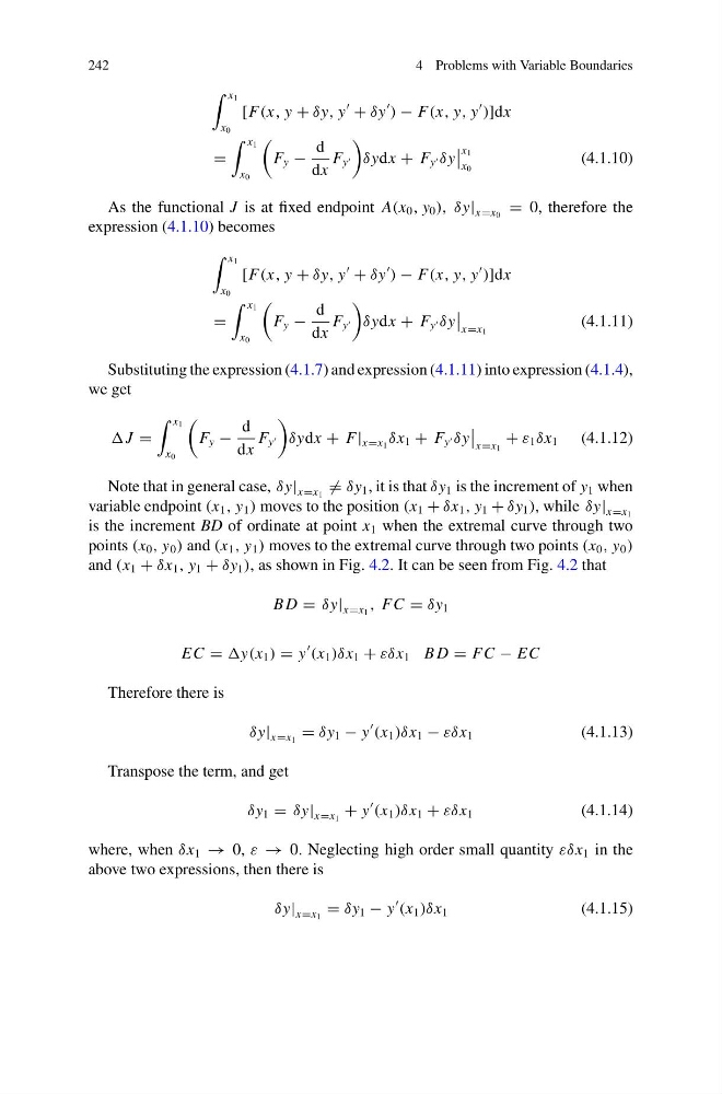
As the functional J is at fixed endpoint A(x 0 , y 0 ), δy| x=x 0 = 0, therefore the
expression (4.1.10) becomes
x 1
x 0
[F(x, y + δy, y
+ δy
) − F(x, y, y
)]dx
=
x 1
x 0
F y −
d
dx
F y
δydx + F y δy
x=x 1
(4.1.11)
Substituting the expression (4.1.7) and expression (4.1.11) into expression (4.1.4),
we get
J =
x 1
x 0
F y −
d
dx
F y
δydx + F| x=x 1 δx 1 + F y δy
x=x 1
+ ε 1 δx 1 (4.1.12)
Note that in general case, δy| x=x 1 = δy 1 , it is that δy 1 is the increment of y 1 when
variable endpoint (x 1 , y 1 ) moves to the position (x 1 + δx 1 , y 1 + δy 1 ), while δy| x=x 1
is the increment BD of ordinate at point x 1 when the extremal curve through two
points (x 0 , y 0 ) and (x 1 , y 1 ) moves to the extremal curve through two points (x 0 , y 0 )
and (x 1 + δx 1 , y 1 + δy 1 ), as shown in Fig. 4.2. It can be seen from Fig. 4.2 that
B D = δy| x=x 1 , FC = δy 1
EC = y(x 1 ) = y
(x 1 )δx 1 + εδx 1 B D = FC − EC
Therefore there is
δy| x=x 1 = δy 1 − y
(x 1 )δx 1 − εδx 1
(4.1.13)
Transpose the term, and get
δy 1 = δy| x=x 1 + y
(x 1 )δx 1 + εδx 1
(4.1.14)
where, when δx 1 → 0, ε → 0. Neglecting high order small quantity εδx 1 in the
above two expressions, then there is
δy| x=x 1 = δy 1 − y
(x 1 )δx 1
(4.1.15)
4 Problems with Variable Boundaries
x 1
x 0
[F(x, y + δy, y
+ δy
) − F(x, y, y
)]dx
=
x 1
x 0
F y −
d
dx
F y
δydx + F y δy
x 1
x 0
(4.1.10)
As the functional J is at fixed endpoint A(x 0 , y 0 ), δy| x=x 0 = 0, therefore the
expression (4.1.10) becomes
x 1
x 0
[F(x, y + δy, y
+ δy
) − F(x, y, y
)]dx
=
x 1
x 0
F y −
d
dx
F y
δydx + F y δy
x=x 1
(4.1.11)
Substituting the expression (4.1.7) and expression (4.1.11) into expression (4.1.4),
we get
J =
x 1
x 0
F y −
d
dx
F y
δydx + F| x=x 1 δx 1 + F y δy
x=x 1
+ ε 1 δx 1 (4.1.12)
Note that in general case, δy| x=x 1 = δy 1 , it is that δy 1 is the increment of y 1 when
variable endpoint (x 1 , y 1 ) moves to the position (x 1 + δx 1 , y 1 + δy 1 ), while δy| x=x 1
is the increment BD of ordinate at point x 1 when the extremal curve through two
points (x 0 , y 0 ) and (x 1 , y 1 ) moves to the extremal curve through two points (x 0 , y 0 )
and (x 1 + δx 1 , y 1 + δy 1 ), as shown in Fig. 4.2. It can be seen from Fig. 4.2 that
B D = δy| x=x 1 , FC = δy 1
EC = y(x 1 ) = y
(x 1 )δx 1 + εδx 1 B D = FC − EC
Therefore there is
δy| x=x 1 = δy 1 − y
(x 1 )δx 1 − εδx 1
(4.1.13)
Transpose the term, and get
δy 1 = δy| x=x 1 + y
(x 1 )δx 1 + εδx 1
(4.1.14)
where, when δx 1 → 0, ε → 0. Neglecting high order small quantity εδx 1 in the
above two expressions, then there is
δy| x=x 1 = δy 1 − y
(x 1 )δx 1
(4.1.15)