

4.1 Variational Problems of the Simplest Functional
243
y ⏐ x =
δy 1
O
x
y
A(x 0 , y 0 )
B(x 1 , y 1 )
C(x 1 + δx 1 , y 1 + δy 1 )
D
E
F
x 0
x 1
x 1 + δx 1
x 1
y = ψ(x)
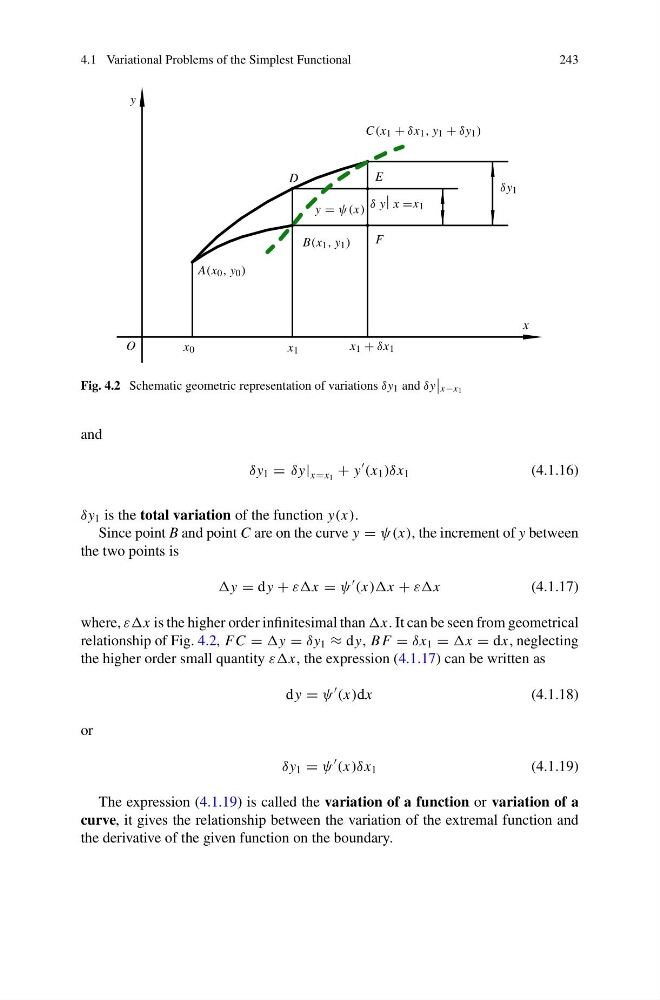
Fig. 4.2 Schematic geometric representation of variations δy 1 and δy
x−x1
and
δy 1 = δy| x=x 1 + y
(x 1 )δx 1
(4.1.16)
δy 1 is the total variation of the function y(x).
Since point B and point C are on the curve y = ψ(x), the increment of y between
the two points is
y = dy + εεx = ψ
(x))x + εεx
(4.1.17)
where, εεx is the higher order infinitesimal than x. It can be seen from geometrical
relationship of Fig. 4.2, FC = y = δy 1 ≈ dy, B F = δx 1 = x = dx, neglecting
the higher order small quantity εεx, the expression (4.1.17) can be written as
dy = ψ
(x)dx
(4.1.18)
or
δy 1 = ψ
(x)δx 1
(4.1.19)
The expression (4.1.19) is called the variation of a function or variation of a
curve, it gives the relationship between the variation of the extremal function and
the derivative of the given function on the boundary.
243
y ⏐ x =
δy 1
O
x
y
A(x 0 , y 0 )
B(x 1 , y 1 )
C(x 1 + δx 1 , y 1 + δy 1 )
D
E
F
x 0
x 1
x 1 + δx 1
x 1
y = ψ(x)
Fig. 4.2 Schematic geometric representation of variations δy 1 and δy
x−x1
and
δy 1 = δy| x=x 1 + y
(x 1 )δx 1
(4.1.16)
δy 1 is the total variation of the function y(x).
Since point B and point C are on the curve y = ψ(x), the increment of y between
the two points is
y = dy + εεx = ψ
(x))x + εεx
(4.1.17)
where, εεx is the higher order infinitesimal than x. It can be seen from geometrical
relationship of Fig. 4.2, FC = y = δy 1 ≈ dy, B F = δx 1 = x = dx, neglecting
the higher order small quantity εεx, the expression (4.1.17) can be written as
dy = ψ
(x)dx
(4.1.18)
or
δy 1 = ψ
(x)δx 1
(4.1.19)
The expression (4.1.19) is called the variation of a function or variation of a
curve, it gives the relationship between the variation of the extremal function and
the derivative of the given function on the boundary.