

216
3 Sufficient Conditions of Extrema of Functionals
3.4 The Legendre Conditions
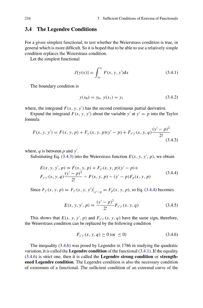
For a given simplest functional, to test whether the Weierstrass condition is true, in
general which is more difficult. So it is hoped that to be able to use a relatively simple
condition replaces the Weierstrass condition.
Let the simplest functional
J [y(x)] =
x 1
x 0
F(x, y, y
)dx
(3.4.1)
The boundary condition is
y(x 0 ) = y 0 , y(x 1 ) = y 1
(3.4.2)
where, the integrand F(x, y, y
) has the second continuous partial derivative.
Expand the integrand F(x, y, y
) about the variable y
at y
= p into the Taylor
formula
F(x, y, y
) = F(x, y, p) + F y (x, y, p)(y
− p) + F y y (x, y, q)
(y
− p)
2
2!
(3.4.3)
where, q is between p and y
.
Substituting Eq. (3.4.3) into the Weierstrass function E(x, y, y
, p), we obtain
E(x, y, y
, p) = F(x, y, p) + F y (x, y, p)(y
− p)+
F y y (x, y, q)
(y
− p)
2
2!
− F(x, y, p) − (y
− p)F p (x, y, p)
(3.4.4)
Since F y (x, y, p) = F y (x, y, y
)
y = p
= F p (x, y, p), so Eq. (3.4.4) becomes
E(x, y, y
, p) =
(y
− p)
2
2!
F y y (x, y, q)
(3.4.5)
This shows that E(x, y, y
, p) and F y y (x, y, q) have the same sign, therefore,
the Weierstrass condition can be replaced by the following condition
F y y (x, y, q) ≥ 0 (or ≤ 0)
(3.4.6)
The inequality (3.4.6) was posed by Legendre in 1786 in studying the quadratic
variation, it is called the Legendre condition of the functional (3.4.1). If the equality
(3.4.6) is strict one, then it is called the Legendre strong condition or strengthened Legendre condition. The Legendre condition is also the necessary condition
of extremum of a functional. The sufficient condition of an extremal curve of the
3 Sufficient Conditions of Extrema of Functionals
3.4 The Legendre Conditions
For a given simplest functional, to test whether the Weierstrass condition is true, in
general which is more difficult. So it is hoped that to be able to use a relatively simple
condition replaces the Weierstrass condition.
Let the simplest functional
J [y(x)] =
x 1
x 0
F(x, y, y
)dx
(3.4.1)
The boundary condition is
y(x 0 ) = y 0 , y(x 1 ) = y 1
(3.4.2)
where, the integrand F(x, y, y
) has the second continuous partial derivative.
Expand the integrand F(x, y, y
) about the variable y
at y
= p into the Taylor
formula
F(x, y, y
) = F(x, y, p) + F y (x, y, p)(y
− p) + F y y (x, y, q)
(y
− p)
2
2!
(3.4.3)
where, q is between p and y
.
Substituting Eq. (3.4.3) into the Weierstrass function E(x, y, y
, p), we obtain
E(x, y, y
, p) = F(x, y, p) + F y (x, y, p)(y
− p)+
F y y (x, y, q)
(y
− p)
2
2!
− F(x, y, p) − (y
− p)F p (x, y, p)
(3.4.4)
Since F y (x, y, p) = F y (x, y, y
)
y = p
= F p (x, y, p), so Eq. (3.4.4) becomes
E(x, y, y
, p) =
(y
− p)
2
2!
F y y (x, y, q)
(3.4.5)
This shows that E(x, y, y
, p) and F y y (x, y, q) have the same sign, therefore,
the Weierstrass condition can be replaced by the following condition
F y y (x, y, q) ≥ 0 (or ≤ 0)
(3.4.6)
The inequality (3.4.6) was posed by Legendre in 1786 in studying the quadratic
variation, it is called the Legendre condition of the functional (3.4.1). If the equality
(3.4.6) is strict one, then it is called the Legendre strong condition or strengthened Legendre condition. The Legendre condition is also the necessary condition
of extremum of a functional. The sufficient condition of an extremal curve of the