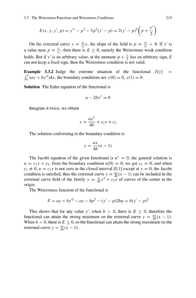
3.3 The Weierstrass Functions and Weierstrass Conditions
215
E(x, y, y
, p) = y
3
− p
3
− 3 p
2
(y
− p) = 2(y
− p)
2
p +
y
2
On the extremal curve y =
y 1
x 1
x, the slope of the field is p =
y 1
x 1
> 0. If y
is
a value near p =
y 1
x 1
, then there is E ≥ 0, namely the Weierstrass weak condition
holds. But if y
is an arbitrary value, at the moment p +
y
2
has an arbitrary sign, E
can not keep a fixed sign, then the Weierstrass condition is not valid.
Example 3.3.2 Judge the extreme situation of the functional J [y] =
1
0 (ay + by
2
)dx, the boundary conditions are y(0) = 0, y(1) = 0.
Solution The Euler equation of the functional is
a − 2by
= 0
Integrate it twice, we obtain
y =
ax
2
4b
+ c 1 x + c 2
The solution conforming to the boundary condition is
y =
ax
4b
(x − 1)
The Jacobi equation of the given functional is u
= 0, the general solution is
u = c 1 x + c 2 . from the boundary condition u(0) = 0, we get c 2 = 0, and when
c 1 = 0, u = c 1 x is not zero in the closed interval [0,1] except at x = 0, the Jacobi
condition is satisfied, thus the extremal curve y =
ax
4b
(x − 1) can be included in the
extremal curve field of the family y =
a
4b
x
2
+ c 2 x of curves of the center at the
origin.
The Weierstrass function of the functional is
E = ay + by
2
− ay − bp
2
− (y
− p)2bp = b(y
− p)
2
This shows that for any value y
, when b > 0, there is E ≥ 0, therefore the
functional can attain the strong minimum on the extremal curve y =
ax
4b
(x − 1).
When b < 0, there is E ≤ 0, so the functional can attain the strong maximum on the
extremal curve y =
ax
4b
(x − 1).