

3.4 The Legendre Conditions
217
functional included in the extremal curve field is which must satisfy the Legendre
strong condition.
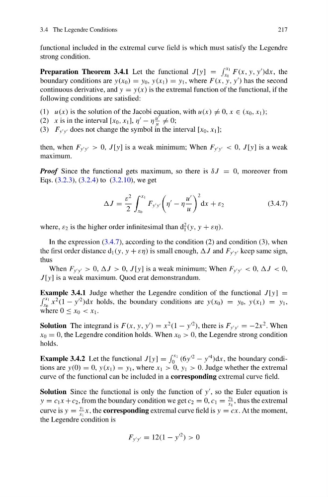
Preparation Theorem 3.4.1 Let the functional J [y] =
x 1
x 0
F(x, y, y
)dx, the
boundary conditions are y(x 0 ) = y 0 , y(x 1 ) = y 1 , where F(x, y, y
) has the second
continuous derivative, and y = y(x) is the extremal function of the functional, if the
following conditions are satisfied:
(1) u(x) is the solution of the Jacobi equation, with u(x) = 0, x ∈ (x 0 , x 1 );
(2) x is in the interval [x 0 , x 1 ], η
− η
u
u
= 0;
(3) F y y does not change the symbol in the interval [x 0 , x 1 ];
then, when F y y > 0, J [y] is a weak minimum; When F y y < 0, J [y] is a weak
maximum.
Proof Since the functional gets maximum, so there is δ J = 0, moreover from
Eqs. (3.2.3), (3.2.4) to (3.2.10), we get
J =
ε
2
2
x 1
x 0
F y y
η
− η
u
u
2
dx + ε 2
(3.4.7)
where, ε 2 is the higher order infinitesimal than d
2
1 (y, y + εη).
In the expression (3.4.7), according to the condition (2) and condition (3), when
the first order distance d 1 (y, y + εη) is small enough, J and F y y keep same sign,
thus
When F y y > 0, J > 0, J [y] is a weak minimum; When F y y < 0, J < 0,
J [y] is a weak maximum. Quod erat demonstrandum.
Example 3.4.1 Judge whether the Legendre condition of the functional J [y] =
x 1
x 0
x
2
(1 − y
2
)dx holds, the boundary conditions are y(x 0 ) = y 0 , y(x 1 ) = y 1 ,
where 0 ≤ x 0 < x 1 .
Solution The integrand is F(x, y, y
) = x
2
(1 − y
2
), there is F y y = −2x
2 . When
x 0 = 0, the Legendre condition holds. When x 0 > 0, the Legendre strong condition
holds.
Example 3.4.2 Let the functional J [y] =
x 1
0 (6y
2
− y
4
)dx, the boundary conditions are y(0) = 0, y(x 1 ) = y 1 , where x 1 > 0, y 1 > 0. Judge whether the extremal
curve of the functional can be included in a corresponding extremal curve field.
Solution Since the functional is only the function of y
, so the Euler equation is
y = c 1 x + c 2 , from the boundary condition we get c 2 = 0, c 1 =
y 1
x 1
, thus the extremal
curve is y =
y 1
x 1
x, the corresponding extremal curve field is y = cx. At the moment,
the Legendre condition is
F y y = 12(1 − y
2
) > 0
217
functional included in the extremal curve field is which must satisfy the Legendre
strong condition.
Preparation Theorem 3.4.1 Let the functional J [y] =
x 1
x 0
F(x, y, y
)dx, the
boundary conditions are y(x 0 ) = y 0 , y(x 1 ) = y 1 , where F(x, y, y
) has the second
continuous derivative, and y = y(x) is the extremal function of the functional, if the
following conditions are satisfied:
(1) u(x) is the solution of the Jacobi equation, with u(x) = 0, x ∈ (x 0 , x 1 );
(2) x is in the interval [x 0 , x 1 ], η
− η
u
u
= 0;
(3) F y y does not change the symbol in the interval [x 0 , x 1 ];
then, when F y y > 0, J [y] is a weak minimum; When F y y < 0, J [y] is a weak
maximum.
Proof Since the functional gets maximum, so there is δ J = 0, moreover from
Eqs. (3.2.3), (3.2.4) to (3.2.10), we get
J =
ε
2
2
x 1
x 0
F y y
η
− η
u
u
2
dx + ε 2
(3.4.7)
where, ε 2 is the higher order infinitesimal than d
2
1 (y, y + εη).
In the expression (3.4.7), according to the condition (2) and condition (3), when
the first order distance d 1 (y, y + εη) is small enough, J and F y y keep same sign,
thus
When F y y > 0, J > 0, J [y] is a weak minimum; When F y y < 0, J < 0,
J [y] is a weak maximum. Quod erat demonstrandum.
Example 3.4.1 Judge whether the Legendre condition of the functional J [y] =
x 1
x 0
x
2
(1 − y
2
)dx holds, the boundary conditions are y(x 0 ) = y 0 , y(x 1 ) = y 1 ,
where 0 ≤ x 0 < x 1 .
Solution The integrand is F(x, y, y
) = x
2
(1 − y
2
), there is F y y = −2x
2 . When
x 0 = 0, the Legendre condition holds. When x 0 > 0, the Legendre strong condition
holds.
Example 3.4.2 Let the functional J [y] =
x 1
0 (6y
2
− y
4
)dx, the boundary conditions are y(0) = 0, y(x 1 ) = y 1 , where x 1 > 0, y 1 > 0. Judge whether the extremal
curve of the functional can be included in a corresponding extremal curve field.
Solution Since the functional is only the function of y
, so the Euler equation is
y = c 1 x + c 2 , from the boundary condition we get c 2 = 0, c 1 =
y 1
x 1
, thus the extremal
curve is y =
y 1
x 1
x, the corresponding extremal curve field is y = cx. At the moment,
the Legendre condition is
F y y = 12(1 − y
2
) > 0