

3.2 The Jacobi Conditions and Jacobi Equation
211
The general solution is
u(x) = d 1 sinh kx + d 2 cosh kx
From the left endpoint condition A(0, 0), we work out d 2 = 0, thus u(x) =
d 1 sinh kx, namely the solution of the Jacobi equation only has one zero. For any
value x 1 being not zero, the Jacobi condition all holds.
3.3 The Weierstrass Functions and Weierstrass Conditions
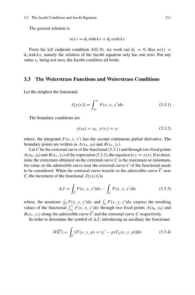
Let the simplest the functional
J [y(x)] =
x 1
x 0
F(x, y, y
)dx
(3.3.1)
The boundary conditions are
y(x 0 ) = y 0 , y(x 1 ) = y 1
(3.3.2)
where, the integrand F(x, y, y
) has the second continuous partial derivative. The
boundary points are written as A(x 0 , y 0 ) and B(x 1 , y 1 ).
Let C be the extremal curve of the functional (3.3.1) and through two fixed points
A(x 0 , y 0 ) and B(x 1 , y 1 ) of the expression (3.3.2), the equation is y = y(x). If to determine the extremum obtained on the extremal curve C is the maximum or minimum,
the value on the admissible curve near the extremal curve C of the functional needs
to be considered. When the extremal curve transits to the admissible curve C near
C, the increment of the functional J [y(x)] is
J =
C
F(x, y, y
)dx −
C
F(x, y, y
)dx
(3.3.3)
where, the notations
C F(x, y, y
)dx and
C F(x, y, y
)dx express the resulting
values of the functional
x 1
x 0
F(x, y, y
)dx through two fixed points A(x 0 , y 0 ) and
B(x 1 , y 1 ) along the admissible curve C and the extremal curve C respectively.
In order to determine the symbol of J , introducing an auxiliary the functional
H [C] =
C
[F(x, y, p) + (y
− p)F p (x, y, p)]dx
(3.3.4)
211
The general solution is
u(x) = d 1 sinh kx + d 2 cosh kx
From the left endpoint condition A(0, 0), we work out d 2 = 0, thus u(x) =
d 1 sinh kx, namely the solution of the Jacobi equation only has one zero. For any
value x 1 being not zero, the Jacobi condition all holds.
3.3 The Weierstrass Functions and Weierstrass Conditions
Let the simplest the functional
J [y(x)] =
x 1
x 0
F(x, y, y
)dx
(3.3.1)
The boundary conditions are
y(x 0 ) = y 0 , y(x 1 ) = y 1
(3.3.2)
where, the integrand F(x, y, y
) has the second continuous partial derivative. The
boundary points are written as A(x 0 , y 0 ) and B(x 1 , y 1 ).
Let C be the extremal curve of the functional (3.3.1) and through two fixed points
A(x 0 , y 0 ) and B(x 1 , y 1 ) of the expression (3.3.2), the equation is y = y(x). If to determine the extremum obtained on the extremal curve C is the maximum or minimum,
the value on the admissible curve near the extremal curve C of the functional needs
to be considered. When the extremal curve transits to the admissible curve C near
C, the increment of the functional J [y(x)] is
J =
C
F(x, y, y
)dx −
C
F(x, y, y
)dx
(3.3.3)
where, the notations
C F(x, y, y
)dx and
C F(x, y, y
)dx express the resulting
values of the functional
x 1
x 0
F(x, y, y
)dx through two fixed points A(x 0 , y 0 ) and
B(x 1 , y 1 ) along the admissible curve C and the extremal curve C respectively.
In order to determine the symbol of J , introducing an auxiliary the functional
H [C] =
C
[F(x, y, p) + (y
− p)F p (x, y, p)]dx
(3.3.4)