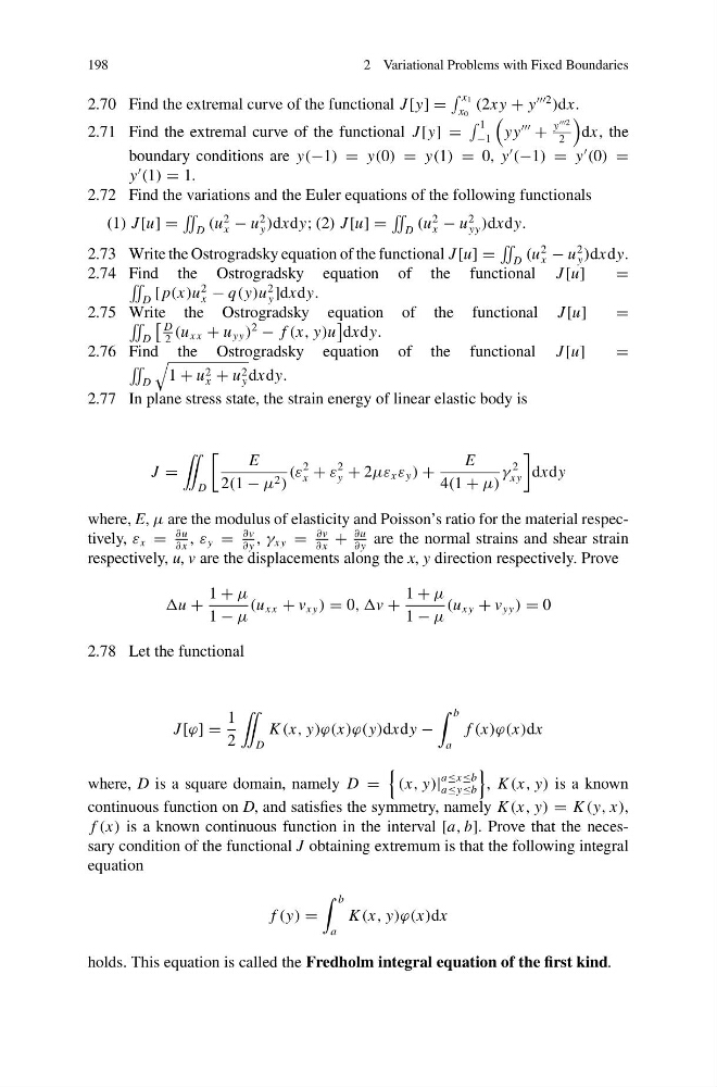
198
2 Variational Problems with Fixed Boundaries
2.70 Find the extremal curve of the functional J [y] =
x 1
x 0
(2x y + y
2
)dx.
2.71 Find the extremal curve of the functional J [y] =
1
−1
yy
+
y
2
2
dx, the
boundary conditions are y(−1) = y(0) = y(1) = 0, y
(−1) = y
(0) =
y
(1) = 1.
2.72 Find the variations and the Euler equations of the following functionals
(1) J [u] =
˜
D (u
2
x − u
2
y )dxdy; (2) J [u] =
˜
D (u
2
x − u
2
yy )dxdy.
2.73 Write the Ostrogradsky equation of the functional J [u] =
˜
D (u
2
x − u
2
y )dxdy.
2.74 Find the Ostrogradsky equation of the functional J [u]
=
˜
D [ p(x)u
2
x − q(y)u
2
y ]dxdy.
2.75 Write the Ostrogradsky equation of the functional J [u]
=
˜
D
D
2
(u xx + u yy )
2
− f (x, y)u
dxdy.
2.76 Find the Ostrogradsky equation of the functional J [u]
=
˜
D
1 + u 2
x + u 2
y dxdy.
2.77 In plane stress state, the strain energy of linear elastic body is
J =
¨
D
E
2(1 − μ 2 )
(ε
2
x + ε
2
y + 2με x ε y ) +
E
4(1 + μ)
γ
2
xy
dxdy
where, E, μ are the modulus of elasticity and Poisson’s ratio for the material respectively, ε x =
∂u
∂ x
, ε y =
∂v
∂ y
, γ xy =
∂v
∂ x
+
∂u
∂ y
are the normal strains and shear strain
respectively, u, v are the displacements along the x, y direction respectively. Prove
u +
1 + μ
1 − μ
(u xx + v xy ) = 0, ,v +
1 + μ
1 − μ
(u xy + v yy ) = 0
2.78 Let the functional
J [ϕ] =
1
2
¨
D
K (x, y)ϕ(x)ϕ(y)dxdy −
b
a
f (x)ϕ(x)dx
where, D is a square domain, namely D =
(x, y)|
a≤x≤b
a≤y≤b
, K (x, y) is a known
continuous function on D, and satisfies the symmetry, namely K (x, y) = K (y, x),
f (x) is a known continuous function in the interval [a, b]. Prove that the necessary condition of the functional J obtaining extremum is that the following integral
equation
f (y) =
b
a
K (x, y)ϕ(x)dx
holds. This equation is called the Fredholm integral equation of the first kind.