

2.8 Variational Problems Depending on Functions of Several Variables
167
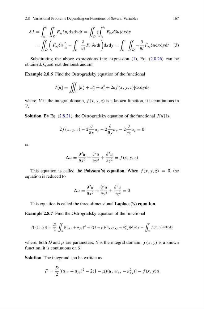
δ J =
t 1
t 0
¨
D
F u t δu t dxdydt =
¨
D
(
t 1
t 0
F u t dδu)dxdy
=
¨
D
F u t δu
t 1
t 0
−
t 1
t 0
∂
∂t
F u t δudt
dxdy =
t 1
t 0
¨
D
−
∂
∂t
F u t δudxdydt (3)
Substituting the above expressions into expression (1), Eq. (2.8.26) can be
obtained. Quod erat demonstrandum.
Example 2.8.6 Find the Ostrogradsky equation of the functional
J [u] =
˚
V
[u
2
x + u
2
y + u
2
z + 2u f (x, y, z)]dxdydz
where, V is the integral domain, f (x, y, z) is a known function, it is continuous in
V.
Solution By Eq. (2.8.21), the Ostrogradsky equation of the functional J [u] is
2 f (x, y, z) − 2
∂
∂ x
u x − 2
∂
∂ y
u y − 2
∂
∂z
u z = 0
or
u =
∂
2 u
∂ x 2 +
∂
2 u
∂ y 2 +
∂
2 u
∂z 2 = f (x, y, z)
This equation is called the Poisson(’s) equation. When f (x, y, z) = 0, the
equation is reduced to
u =
∂
2 u
∂ x 2 +
∂
2 u
∂ y 2 +
∂
2 u
∂z 2 = 0
This equation is called the three-dimensional Laplace(’s) equation.
Example 2.8.7 Find the Ostrogradsky equation of the functional
J [u(x, y)] =
D
2
¨
S
[(u xx + u yy )
2 − 2(1 − μ)(u xx u yy − u
2
xy )]dxdy −
¨
S
f (x, y)udxdy
where, both D and μ are parameters; S is the integral domain; f (x, y) is a known
function, it is continuous on S.
Solution The integrand can be written as
F =
D
2
[(u xx + u yy )
2
− 2(1 − μ)(u xx u yy − u
2
xy )] − f (x, y)u
167
δ J =
t 1
t 0
¨
D
F u t δu t dxdydt =
¨
D
(
t 1
t 0
F u t dδu)dxdy
=
¨
D
F u t δu
t 1
t 0
−
t 1
t 0
∂
∂t
F u t δudt
dxdy =
t 1
t 0
¨
D
−
∂
∂t
F u t δudxdydt (3)
Substituting the above expressions into expression (1), Eq. (2.8.26) can be
obtained. Quod erat demonstrandum.
Example 2.8.6 Find the Ostrogradsky equation of the functional
J [u] =
˚
V
[u
2
x + u
2
y + u
2
z + 2u f (x, y, z)]dxdydz
where, V is the integral domain, f (x, y, z) is a known function, it is continuous in
V.
Solution By Eq. (2.8.21), the Ostrogradsky equation of the functional J [u] is
2 f (x, y, z) − 2
∂
∂ x
u x − 2
∂
∂ y
u y − 2
∂
∂z
u z = 0
or
u =
∂
2 u
∂ x 2 +
∂
2 u
∂ y 2 +
∂
2 u
∂z 2 = f (x, y, z)
This equation is called the Poisson(’s) equation. When f (x, y, z) = 0, the
equation is reduced to
u =
∂
2 u
∂ x 2 +
∂
2 u
∂ y 2 +
∂
2 u
∂z 2 = 0
This equation is called the three-dimensional Laplace(’s) equation.
Example 2.8.7 Find the Ostrogradsky equation of the functional
J [u(x, y)] =
D
2
¨
S
[(u xx + u yy )
2 − 2(1 − μ)(u xx u yy − u
2
xy )]dxdy −
¨
S
f (x, y)udxdy
where, both D and μ are parameters; S is the integral domain; f (x, y) is a known
function, it is continuous on S.
Solution The integrand can be written as
F =
D
2
[(u xx + u yy )
2
− 2(1 − μ)(u xx u yy − u
2
xy )] − f (x, y)u