

168
2 Variational Problems with Fixed Boundaries
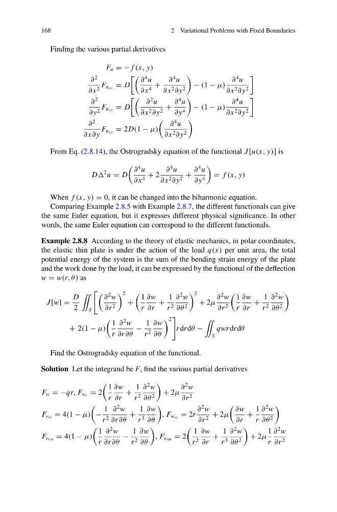
Finding the various partial derivatives
F u = − f (x, y)
∂
2
∂ x 2 F u xx = D
∂
4 u
∂ x 4 +
∂
4 u
∂ x 2 ∂ y 2
− (1 − μ)
∂
4 u
∂ x 2 ∂ y 2
∂
2
∂ y 2 F u yy = D
∂
2 u
∂ x 2 ∂ y 2 +
∂
4 u
∂ y 4
− (1 − μ)
∂
4 u
∂ x 2 ∂ y 2
∂
2
∂ x∂ y
F u xy = 2D(1 − μ)
∂
4 u
∂ x 2 ∂ y 2
From Eq. (2.8.14), the Ostrogradsky equation of the functional J [u(x, y)] is
D
2 u = D
∂
4 u
∂ x 4 + 2
∂
4 u
∂ x 2 ∂ y 2 +
∂
4 u
∂ y 4
= f (x, y)
When f (x, y) = 0, it can be changed into the biharmonic equation.
Comparing Example 2.8.5 with Example 2.8.7, the different functionals can give
the same Euler equation, but it expresses different physical significance. In other
words, the same Euler equation can correspond to the different functionals.
Example 2.8.8 According to the theory of elastic mechanics, in polar coordinates,
the elastic thin plate is under the action of the load q(x) per unit area, the total
potential energy of the system is the sum of the bending strain energy of the plate
and the work done by the load, it can be expressed by the functional of the deflection
w = w(r, θ) as
J [w] =
D
2
¨
S
∂
2 w
∂r 2
2
+
1
r
∂w
∂r
+
1
r 2
∂
2 w
∂θ 2
2
+ 2μ
∂
2 w
∂r 2
1
r
∂w
∂r
+
1
r 2
∂
2 w
∂θ 2
+ 2(1 − μ)
1
r
∂
2 w
∂r ∂θ
−
1
r 2
∂w
∂θ
2
r dr dθ −
¨
S
qwrdr dθ
Find the Ostrogradsky equation of the functional.
Solution Let the integrand be F, find the various partial derivatives
F w = −qr, F w r = 2
1
r
∂w
∂r
+
1
r 2
∂
2 w
∂θ 2
+ 2μ
∂
2 w
∂r 2
F w θ = 4(1 − μ)
−
1
r 2
∂
2 w
∂r ∂θ
+
1
r 3
∂w
∂θ
, F w rr = 2r
∂
2 w
∂r 2 + 2μ
∂w
∂r
+
1
r
∂
2 w
∂θ 2
F w r θ = 4(1 − μ)
1
r
∂
2 w
∂r ∂θ
−
1
r 2
∂w
∂θ
, F w θθ = 2
1
r 2
∂w
∂r
+
1
r 3
∂
2 w
∂θ 2
+ 2μ
1
r
∂
2 w
∂r 2
2 Variational Problems with Fixed Boundaries
Finding the various partial derivatives
F u = − f (x, y)
∂
2
∂ x 2 F u xx = D
∂
4 u
∂ x 4 +
∂
4 u
∂ x 2 ∂ y 2
− (1 − μ)
∂
4 u
∂ x 2 ∂ y 2
∂
2
∂ y 2 F u yy = D
∂
2 u
∂ x 2 ∂ y 2 +
∂
4 u
∂ y 4
− (1 − μ)
∂
4 u
∂ x 2 ∂ y 2
∂
2
∂ x∂ y
F u xy = 2D(1 − μ)
∂
4 u
∂ x 2 ∂ y 2
From Eq. (2.8.14), the Ostrogradsky equation of the functional J [u(x, y)] is
D
2 u = D
∂
4 u
∂ x 4 + 2
∂
4 u
∂ x 2 ∂ y 2 +
∂
4 u
∂ y 4
= f (x, y)
When f (x, y) = 0, it can be changed into the biharmonic equation.
Comparing Example 2.8.5 with Example 2.8.7, the different functionals can give
the same Euler equation, but it expresses different physical significance. In other
words, the same Euler equation can correspond to the different functionals.
Example 2.8.8 According to the theory of elastic mechanics, in polar coordinates,
the elastic thin plate is under the action of the load q(x) per unit area, the total
potential energy of the system is the sum of the bending strain energy of the plate
and the work done by the load, it can be expressed by the functional of the deflection
w = w(r, θ) as
J [w] =
D
2
¨
S
∂
2 w
∂r 2
2
+
1
r
∂w
∂r
+
1
r 2
∂
2 w
∂θ 2
2
+ 2μ
∂
2 w
∂r 2
1
r
∂w
∂r
+
1
r 2
∂
2 w
∂θ 2
+ 2(1 − μ)
1
r
∂
2 w
∂r ∂θ
−
1
r 2
∂w
∂θ
2
r dr dθ −
¨
S
qwrdr dθ
Find the Ostrogradsky equation of the functional.
Solution Let the integrand be F, find the various partial derivatives
F w = −qr, F w r = 2
1
r
∂w
∂r
+
1
r 2
∂
2 w
∂θ 2
+ 2μ
∂
2 w
∂r 2
F w θ = 4(1 − μ)
−
1
r 2
∂
2 w
∂r ∂θ
+
1
r 3
∂w
∂θ
, F w rr = 2r
∂
2 w
∂r 2 + 2μ
∂w
∂r
+
1
r
∂
2 w
∂θ 2
F w r θ = 4(1 − μ)
1
r
∂
2 w
∂r ∂θ
−
1
r 2
∂w
∂θ
, F w θθ = 2
1
r 2
∂w
∂r
+
1
r 3
∂
2 w
∂θ 2
+ 2μ
1
r
∂
2 w
∂r 2