

2.7 Variational Problems Depending on Higher Order Derivatives
153
n
k=1
(−1)
k−1 d
k−1
dy k−1 ϕ x (k) = ϕ x −
d
dy
ϕ x + · · · + (−1)
n−1 d
n−1
dy n−1 ϕ x (n) = c (2.7.26)
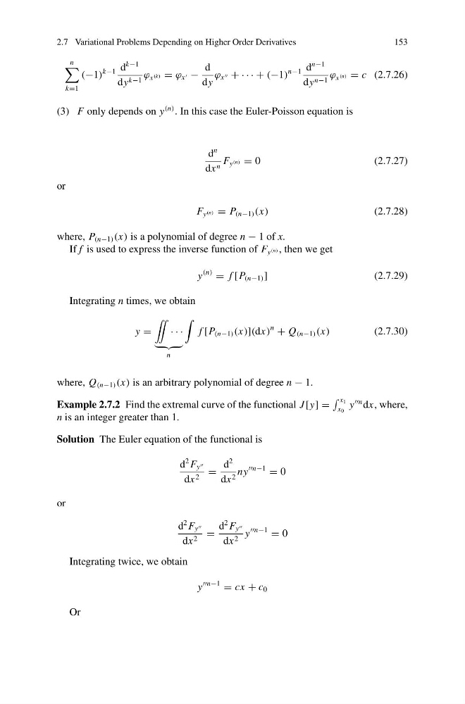
(3) F only depends on y
(n) . In this case the Euler-Poisson equation is
d
n
dx n F y (n) = 0
(2.7.27)
or
F y (n) = P (n−1) (x)
(2.7.28)
where, P (n−1) (x) is a polynomial of degree n − 1 of x.
If f is used to express the inverse function of F y (n) , then we get
y
(n)
= f [P (n−1) ]
(2.7.29)
Integrating n times, we obtain
y =
¨
· · ·
n
f [P (n−1) (x)](dx)
n
+ Q (n−1) (x)
(2.7.30)
where, Q (n−1) (x) is an arbitrary polynomial of degree n − 1.
Example 2.7.2 Find the extremal curve of the functional J [y] =
x 1
x 0
y
n dx, where,
n is an integer greater than 1.
Solution The Euler equation of the functional is
d
2 F y
dx 2 =
d
2
dx 2 ny
n−1
= 0
or
d
2 F y
dx 2 =
d
2 F y
dx 2 y
n−1
= 0
Integrating twice, we obtain
y
n−1
= cx + c 0
Or
153
n
k=1
(−1)
k−1 d
k−1
dy k−1 ϕ x (k) = ϕ x −
d
dy
ϕ x + · · · + (−1)
n−1 d
n−1
dy n−1 ϕ x (n) = c (2.7.26)
(3) F only depends on y
(n) . In this case the Euler-Poisson equation is
d
n
dx n F y (n) = 0
(2.7.27)
or
F y (n) = P (n−1) (x)
(2.7.28)
where, P (n−1) (x) is a polynomial of degree n − 1 of x.
If f is used to express the inverse function of F y (n) , then we get
y
(n)
= f [P (n−1) ]
(2.7.29)
Integrating n times, we obtain
y =
¨
· · ·
n
f [P (n−1) (x)](dx)
n
+ Q (n−1) (x)
(2.7.30)
where, Q (n−1) (x) is an arbitrary polynomial of degree n − 1.
Example 2.7.2 Find the extremal curve of the functional J [y] =
x 1
x 0
y
n dx, where,
n is an integer greater than 1.
Solution The Euler equation of the functional is
d
2 F y
dx 2 =
d
2
dx 2 ny
n−1
= 0
or
d
2 F y
dx 2 =
d
2 F y
dx 2 y
n−1
= 0
Integrating twice, we obtain
y
n−1
= cx + c 0
Or