

154
2 Variational Problems with Fixed Boundaries
y
= (cx + c 0 )
1
n−1
Integrating twice again, we obtain
y = (c 1 x + c 2 )
2n−1
n−1 + c 3 x + c 4
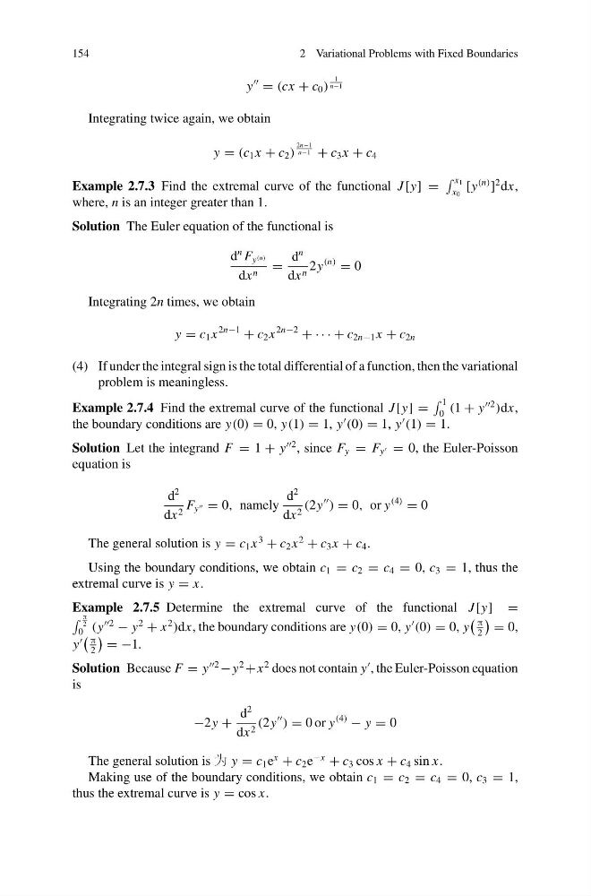
Example 2.7.3 Find the extremal curve of the functional J [y] =
x 1
x 0
[y
(n)
]
2 dx,
where, n is an integer greater than 1.
Solution The Euler equation of the functional is
d
n F y (n)
dx n =
d
n
dx n 2y
(n)
= 0
Integrating 2n times, we obtain
y = c 1 x
2n−1
+ c 2 x
2n−2
+ · · · + c 2n−1 x + c 2n
(4) If under the integral sign is the total differential of a function, then the variational
problem is meaningless.
Example 2.7.4 Find the extremal curve of the functional J [y] =
1
0 (1 + y
2
)dx,
the boundary conditions are y(0) = 0, y(1) = 1, y
(0) = 1, y
(1) = 1.
Solution Let the integrand F = 1 + y
2 , since F y = F y = 0, the Euler-Poisson
equation is
d
2
dx 2 F y = 0, namely
d
2
dx 2 (2y
) = 0, or y
(4)
= 0
The general solution is y = c 1 x
3
+ c 2 x
2
+ c 3 x + c 4 .
Using the boundary conditions, we obtain c 1 = c 2 = c 4 = 0, c 3 = 1, thus the
extremal curve is y = x.
Example 2.7.5 Determine the extremal curve of the functional J [y] =
π
2
0 (y
2
− y
2
+ x
2
)dx, the boundary conditions are y(0) = 0, y
(0) = 0, y
π
2
= 0,
y
π
2
= −1.
Solution Because F = y
2
− y
2
+x
2 does not contain y
, the Euler-Poisson equation
is
−2y +
d
2
dx 2 (2y
) = 0 or y
(4)
− y = 0
The general solution is 为 y = c 1 e
x
+ c 2 e
−x
+ c 3 cos x + c 4 sin x.
Making use of the boundary conditions, we obtain c 1 = c 2 = c 4 = 0, c 3 = 1,
thus the extremal curve is y = cos x.
2 Variational Problems with Fixed Boundaries
y
= (cx + c 0 )
1
n−1
Integrating twice again, we obtain
y = (c 1 x + c 2 )
2n−1
n−1 + c 3 x + c 4
Example 2.7.3 Find the extremal curve of the functional J [y] =
x 1
x 0
[y
(n)
]
2 dx,
where, n is an integer greater than 1.
Solution The Euler equation of the functional is
d
n F y (n)
dx n =
d
n
dx n 2y
(n)
= 0
Integrating 2n times, we obtain
y = c 1 x
2n−1
+ c 2 x
2n−2
+ · · · + c 2n−1 x + c 2n
(4) If under the integral sign is the total differential of a function, then the variational
problem is meaningless.
Example 2.7.4 Find the extremal curve of the functional J [y] =
1
0 (1 + y
2
)dx,
the boundary conditions are y(0) = 0, y(1) = 1, y
(0) = 1, y
(1) = 1.
Solution Let the integrand F = 1 + y
2 , since F y = F y = 0, the Euler-Poisson
equation is
d
2
dx 2 F y = 0, namely
d
2
dx 2 (2y
) = 0, or y
(4)
= 0
The general solution is y = c 1 x
3
+ c 2 x
2
+ c 3 x + c 4 .
Using the boundary conditions, we obtain c 1 = c 2 = c 4 = 0, c 3 = 1, thus the
extremal curve is y = x.
Example 2.7.5 Determine the extremal curve of the functional J [y] =
π
2
0 (y
2
− y
2
+ x
2
)dx, the boundary conditions are y(0) = 0, y
(0) = 0, y
π
2
= 0,
y
π
2
= −1.
Solution Because F = y
2
− y
2
+x
2 does not contain y
, the Euler-Poisson equation
is
−2y +
d
2
dx 2 (2y
) = 0 or y
(4)
− y = 0
The general solution is 为 y = c 1 e
x
+ c 2 e
−x
+ c 3 cos x + c 4 sin x.
Making use of the boundary conditions, we obtain c 1 = c 2 = c 4 = 0, c 3 = 1,
thus the extremal curve is y = cos x.