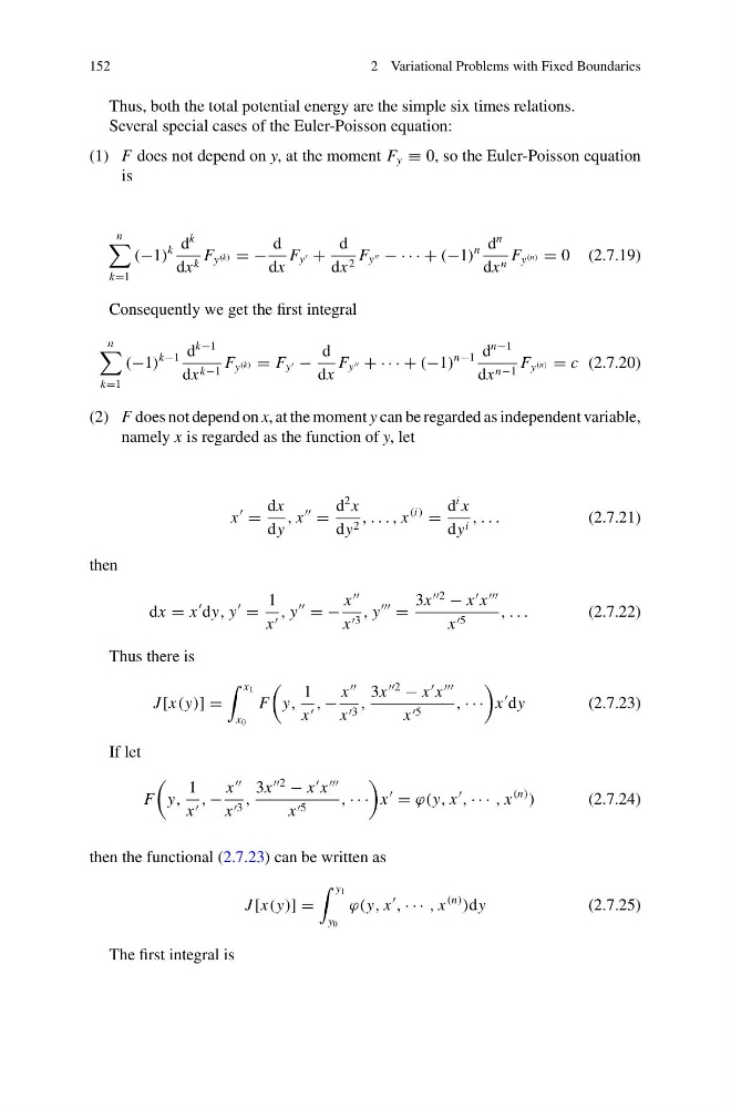
152
2 Variational Problems with Fixed Boundaries
Thus, both the total potential energy are the simple six times relations.
Several special cases of the Euler-Poisson equation:
(1) F does not depend on y, at the moment F y ≡ 0, so the Euler-Poisson equation
is
n
k=1
(−1)
k d
k
dx k F y (k) = −
d
dx
F y +
d
dx 2 F y − · · · + (−1)
n d
n
dx n F y (n) = 0 (2.7.19)
Consequently we get the first integral
n
k=1
(−1)
k−1 d
k−1
dx k−1 F y (k) = F y −
d
dx
F y + · · · + (−1)
n−1 d
n−1
dx n−1 F y (n) = c (2.7.20)
(2) F does not depend on x, at the moment y can be regarded as independent variable,
namely x is regarded as the function of y, let
x
=
dx
dy
, x
=
d
2 x
dy 2 , . . . , x
(i)
=
d
i x
dy i , . . .
(2.7.21)
then
dx = x
dy, y
=
1
x , y
= −
x
x 3 , y
=
3x
2
− x
x
x 5
, . . .
(2.7.22)
Thus there is
J [x(y)] =
x 1
x 0
F
y,
1
x , −
x
x 3 ,
3x
2
− x
x
x 5
, · · ·
x
dy
(2.7.23)
If let
F
y,
1
x , −
x
x 3 ,
3x
2
− x
x
x 5
, · · ·
x
= ϕ(y, x
, · · · , x
(n)
)
(2.7.24)
then the functional (2.7.23) can be written as
J [x(y)] =
y 1
y 0
ϕ(y, x
, · · · , x
(n)
)dy
(2.7.25)
The first integral is