

148
2 Variational Problems with Fixed Boundaries
δy|
x 1
x 0 = 0, δy
x 1
x 0
= 0, δ J = 0
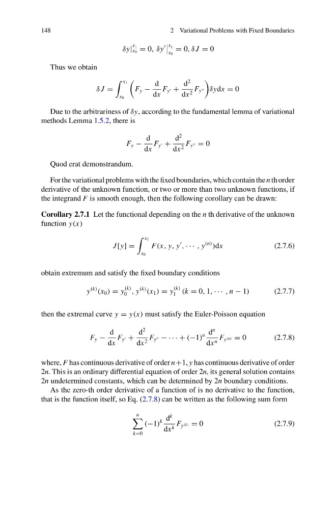
Thus we obtain
δ J =
x 1
x 0
F y −
d
dx
F y +
d
2
dx 2 F y
δydx = 0
Due to the arbitrariness of δy, according to the fundamental lemma of variational
methods Lemma 1.5.2, there is
F y −
d
dx
F y +
d
2
dx 2 F y = 0
Quod erat demonstrandum.
For the variational problems with the fixed boundaries, which contain the n th order
derivative of the unknown function, or two or more than two unknown functions, if
the integrand F is smooth enough, then the following corollary can be drawn:
Corollary 2.7.1 Let the functional depending on the n th derivative of the unknown
function y(x)
J [y] =
x 1
x 0
F(x, y, y
, · · · , y
(n)
)dx
(2.7.6)
obtain extremum and satisfy the fixed boundary conditions
y
(k)
(x 0 ) = y
(k)
0 , y
(k)
(x 1 ) = y
(k)
1 (k = 0, 1, · · · , n − 1)
(2.7.7)
then the extremal curve y = y(x) must satisfy the Euler-Poisson equation
F y −
d
dx
F y +
d
2
dx 2 F y − · · · + (−1)
n d
n
dx n F y (n) = 0
(2.7.8)
where, F has continuous derivative of order n+1, y has continuous derivative of order
2n. This is an ordinary differential equation of order 2n, its general solution contains
2n undetermined constants, which can be determined by 2n boundary conditions.
As the zero-th order derivative of a function of is no derivative to the function,
that is the function itself, so Eq. (2.7.8) can be written as the following sum form
n
k=0
(−1)
k d
k
dx k F y (k) = 0
(2.7.9)
2 Variational Problems with Fixed Boundaries
δy|
x 1
x 0 = 0, δy
x 1
x 0
= 0, δ J = 0
Thus we obtain
δ J =
x 1
x 0
F y −
d
dx
F y +
d
2
dx 2 F y
δydx = 0
Due to the arbitrariness of δy, according to the fundamental lemma of variational
methods Lemma 1.5.2, there is
F y −
d
dx
F y +
d
2
dx 2 F y = 0
Quod erat demonstrandum.
For the variational problems with the fixed boundaries, which contain the n th order
derivative of the unknown function, or two or more than two unknown functions, if
the integrand F is smooth enough, then the following corollary can be drawn:
Corollary 2.7.1 Let the functional depending on the n th derivative of the unknown
function y(x)
J [y] =
x 1
x 0
F(x, y, y
, · · · , y
(n)
)dx
(2.7.6)
obtain extremum and satisfy the fixed boundary conditions
y
(k)
(x 0 ) = y
(k)
0 , y
(k)
(x 1 ) = y
(k)
1 (k = 0, 1, · · · , n − 1)
(2.7.7)
then the extremal curve y = y(x) must satisfy the Euler-Poisson equation
F y −
d
dx
F y +
d
2
dx 2 F y − · · · + (−1)
n d
n
dx n F y (n) = 0
(2.7.8)
where, F has continuous derivative of order n+1, y has continuous derivative of order
2n. This is an ordinary differential equation of order 2n, its general solution contains
2n undetermined constants, which can be determined by 2n boundary conditions.
As the zero-th order derivative of a function of is no derivative to the function,
that is the function itself, so Eq. (2.7.8) can be written as the following sum form
n
k=0
(−1)
k d
k
dx k F y (k) = 0
(2.7.9)