

2.7 Variational Problems Depending on Higher Order Derivatives
147
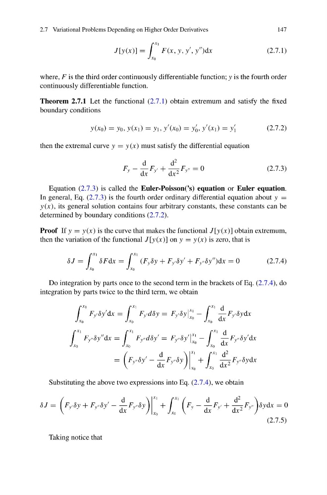
J [y(x)] =
x 1
x 0
F(x, y, y
, y
)dx
(2.7.1)
where, F is the third order continuously differentiable function; y is the fourth order
continuously differentiable function.
Theorem 2.7.1 Let the functional (2.7.1) obtain extremum and satisfy the fixed
boundary conditions
y(x 0 ) = y 0 , y(x 1 ) = y 1 , y
(x 0 ) = y
0 , y
(x 1 ) = y
1
(2.7.2)
then the extremal curve y = y(x) must satisfy the differential equation
F y −
d
dx
F y +
d
2
dx 2 F y = 0
(2.7.3)
Equation (2.7.3) is called the Euler-Poisson(’s) equation or Euler equation.
In general, Eq. (2.7.3) is the fourth order ordinary differential equation about y =
y(x), its general solution contains four arbitrary constants, these constants can be
determined by boundary conditions (2.7.2).
Proof If y = y(x) is the curve that makes the functional J [y(x)] obtain extremum,
then the variation of the functional J [y(x)] on y = y(x) is zero, that is
δ J =
x 1
x 0
δ Fdx =
x 1
x 0
(F y δy + F y δy
+ F y δy
)dx = 0
(2.7.4)
Do integration by parts once to the second term in the brackets of Eq. (2.7.4), do
integration by parts twice to the third term, we obtain
x 1
x 0
F y δy
dx =
x 1
x 0
F y dδy = F y δy
x 1
x 0
−
x 1
x 0
d
dx
F y δydx
x 1
x 0
F y δy
dx =
x 1
x 0
F y dδy
= F y δy
x 1
x 0
−
x 1
x 0
d
dx
F y δy
dx
=
F y δy
−
d
dx
F y δy
x 1
x 0
+
x 1
x 0
d
2
dx 2 F y δydx
Substituting the above two expressions into Eq. (2.7.4), we obtain
δ J =
F y δy + F y δy
−
d
dx
F y δy
x 1
x 0
+
x 1
x 0
F y −
d
dx
F y +
d
2
dx 2 F y
δydx = 0
(2.7.5)
Taking notice that
147
J [y(x)] =
x 1
x 0
F(x, y, y
, y
)dx
(2.7.1)
where, F is the third order continuously differentiable function; y is the fourth order
continuously differentiable function.
Theorem 2.7.1 Let the functional (2.7.1) obtain extremum and satisfy the fixed
boundary conditions
y(x 0 ) = y 0 , y(x 1 ) = y 1 , y
(x 0 ) = y
0 , y
(x 1 ) = y
1
(2.7.2)
then the extremal curve y = y(x) must satisfy the differential equation
F y −
d
dx
F y +
d
2
dx 2 F y = 0
(2.7.3)
Equation (2.7.3) is called the Euler-Poisson(’s) equation or Euler equation.
In general, Eq. (2.7.3) is the fourth order ordinary differential equation about y =
y(x), its general solution contains four arbitrary constants, these constants can be
determined by boundary conditions (2.7.2).
Proof If y = y(x) is the curve that makes the functional J [y(x)] obtain extremum,
then the variation of the functional J [y(x)] on y = y(x) is zero, that is
δ J =
x 1
x 0
δ Fdx =
x 1
x 0
(F y δy + F y δy
+ F y δy
)dx = 0
(2.7.4)
Do integration by parts once to the second term in the brackets of Eq. (2.7.4), do
integration by parts twice to the third term, we obtain
x 1
x 0
F y δy
dx =
x 1
x 0
F y dδy = F y δy
x 1
x 0
−
x 1
x 0
d
dx
F y δydx
x 1
x 0
F y δy
dx =
x 1
x 0
F y dδy
= F y δy
x 1
x 0
−
x 1
x 0
d
dx
F y δy
dx
=
F y δy
−
d
dx
F y δy
x 1
x 0
+
x 1
x 0
d
2
dx 2 F y δydx
Substituting the above two expressions into Eq. (2.7.4), we obtain
δ J =
F y δy + F y δy
−
d
dx
F y δy
x 1
x 0
+
x 1
x 0
F y −
d
dx
F y +
d
2
dx 2 F y
δydx = 0
(2.7.5)
Taking notice that