

2.5 Several Special Cases of the Euler Equation and Their Integrals
133
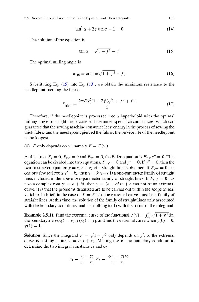
tan
2
α + 2 f tan α − 1 = 0
( 1 4 )
The solution of the equation is
tan α =
1 + f 2 − f
(15)
The optimal milling angle is
α opt = arctan(
1 + f 2 − f )
(16)
Substituting Eq. (15) into Eq. (13), we obtain the minimum resistance to the
needlepoint piercing the fabric
P min =
2πE x
2
1 [1 + 2 f (
1 + f 2 + f )]
3
(17)
Therefore, if the needlepoint is processed into a hyperboloid with the optimal
milling angle or a right circle cone surface under special circumstances, which can
guarantee that the sewing machine consumes least energy in the process of sewing the
thick fabric and the needlepoint pierced the fabric, the service life of the needlepoint
is the longest.
(4) F only depends on y
, namely F = F(y
)
At this time, F y = 0, F xy = 0 and F yy = 0, the Euler equation is F y y y
= 0. This
equation can be divided into two equations, F y y = 0 and y
= 0. If y
= 0, then the
two-parameter equation y = c 1 x + c 2 of a straight line is obtained. If F y y = 0 has
one or a few real roots y
= k i , then y = k i x + c is a one-parameter family of straight
lines included in the above two-parameter family of straight lines. If F y y = 0 has
also a complex root y
= a + bi, then y = (a + bi)x + c can not be an extremal
curve, it is that the problems discussed are to be carried out within the scope of real
variable. In brief, in the case of F = F(y
), the extremal curve must be a family of
straight lines. At this time, the solution of the family of straight lines only associated
with the boundary conditions, and has nothing to do with the forms of the integrand.
Example 2.5.11 Find the extremal curve of the functional J [y] =
x 1
x 0
1 + y 2 dx,
the boundary are y(x 0 ) = y 0 , y(x 1 ) = y 1 , and find the extremal curve when y(0) = 0,
y(1) = 1.
Solution Since the integrand F =
1 + y 2 only depends on y
, so the extremal
curve is a straight line y = c 1 x + c 2 . Making use of the boundary condition to
determine the two integral constants c 1 and c 2
c 1 =
y 1 − y 0
x 1 − x 0
, c 2 =
y 0 x 1 − y 1 x 0
x 1 − x 0
133
tan
2
α + 2 f tan α − 1 = 0
( 1 4 )
The solution of the equation is
tan α =
1 + f 2 − f
(15)
The optimal milling angle is
α opt = arctan(
1 + f 2 − f )
(16)
Substituting Eq. (15) into Eq. (13), we obtain the minimum resistance to the
needlepoint piercing the fabric
P min =
2πE x
2
1 [1 + 2 f (
1 + f 2 + f )]
3
(17)
Therefore, if the needlepoint is processed into a hyperboloid with the optimal
milling angle or a right circle cone surface under special circumstances, which can
guarantee that the sewing machine consumes least energy in the process of sewing the
thick fabric and the needlepoint pierced the fabric, the service life of the needlepoint
is the longest.
(4) F only depends on y
, namely F = F(y
)
At this time, F y = 0, F xy = 0 and F yy = 0, the Euler equation is F y y y
= 0. This
equation can be divided into two equations, F y y = 0 and y
= 0. If y
= 0, then the
two-parameter equation y = c 1 x + c 2 of a straight line is obtained. If F y y = 0 has
one or a few real roots y
= k i , then y = k i x + c is a one-parameter family of straight
lines included in the above two-parameter family of straight lines. If F y y = 0 has
also a complex root y
= a + bi, then y = (a + bi)x + c can not be an extremal
curve, it is that the problems discussed are to be carried out within the scope of real
variable. In brief, in the case of F = F(y
), the extremal curve must be a family of
straight lines. At this time, the solution of the family of straight lines only associated
with the boundary conditions, and has nothing to do with the forms of the integrand.
Example 2.5.11 Find the extremal curve of the functional J [y] =
x 1
x 0
1 + y 2 dx,
the boundary are y(x 0 ) = y 0 , y(x 1 ) = y 1 , and find the extremal curve when y(0) = 0,
y(1) = 1.
Solution Since the integrand F =
1 + y 2 only depends on y
, so the extremal
curve is a straight line y = c 1 x + c 2 . Making use of the boundary condition to
determine the two integral constants c 1 and c 2
c 1 =
y 1 − y 0
x 1 − x 0
, c 2 =
y 0 x 1 − y 1 x 0
x 1 − x 0