

114
2 Variational Problems with Fixed Boundaries
called the Euler-Lagrange(’s) equation. Thus, the calculus of variations formed a
new branch of mathematical analysis. The Euler equation is the variational condition
of a functional in the domain. In the calculus of variations, all of the differential
equations corresponding to the functional with the structure of Eq. (2.4.1) can be
called the Euler equation.
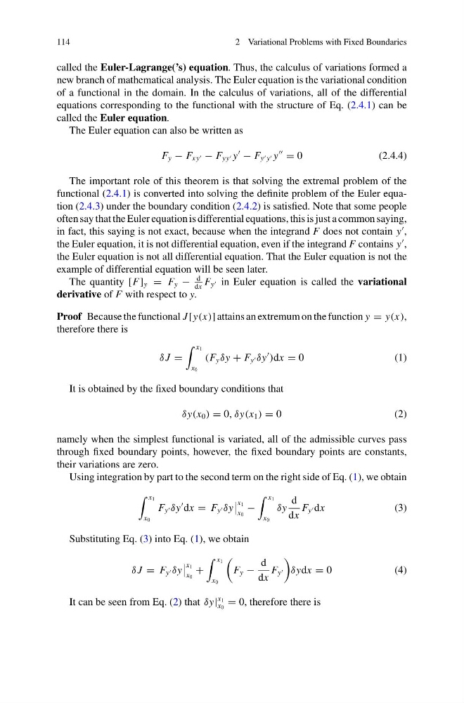
The Euler equation can also be written as
F y − F xy − F yy y
− F y y y
= 0
(2.4.4)
The important role of this theorem is that solving the extremal problem of the
functional (2.4.1) is converted into solving the definite problem of the Euler equation (2.4.3) under the boundary condition (2.4.2) is satisfied. Note that some people
often say that the Euler equation is differential equations, this is just a common saying,
in fact, this saying is not exact, because when the integrand F does not contain y
,
the Euler equation, it is not differential equation, even if the integrand F contains y
,
the Euler equation is not all differential equation. That the Euler equation is not the
example of differential equation will be seen later.
The quantity [F] y = F y −
d
dx
F y in Euler equation is called the variational
derivative of F with respect to y.
Proof Because the functional J [y(x)] attains an extremum on the function y = y(x),
therefore there is
δ J =
x 1
x 0
(F y δy + F y δy
)dx = 0
( 1 )
It is obtained by the fixed boundary conditions that
δy(x 0 ) = 0, δy(x 1 ) = 0
( 2 )
namely when the simplest functional is variated, all of the admissible curves pass
through fixed boundary points, however, the fixed boundary points are constants,
their variations are zero.
Using integration by part to the second term on the right side of Eq. (1), we obtain
x 1
x 0
F y δy
dx = F y δy
x 1
x 0
−
x 1
x 0
δy
d
dx
F y dx
(3)
Substituting Eq. (3) into Eq. (1), we obtain
δ J = F y δy
x 1
x 0
+
x 1
x 0
F y −
d
dx
F y
δydx = 0
( 4 )
It can be seen from Eq. (2) that δy|
x 1
x 0
= 0, therefore there is
2 Variational Problems with Fixed Boundaries
called the Euler-Lagrange(’s) equation. Thus, the calculus of variations formed a
new branch of mathematical analysis. The Euler equation is the variational condition
of a functional in the domain. In the calculus of variations, all of the differential
equations corresponding to the functional with the structure of Eq. (2.4.1) can be
called the Euler equation.
The Euler equation can also be written as
F y − F xy − F yy y
− F y y y
= 0
(2.4.4)
The important role of this theorem is that solving the extremal problem of the
functional (2.4.1) is converted into solving the definite problem of the Euler equation (2.4.3) under the boundary condition (2.4.2) is satisfied. Note that some people
often say that the Euler equation is differential equations, this is just a common saying,
in fact, this saying is not exact, because when the integrand F does not contain y
,
the Euler equation, it is not differential equation, even if the integrand F contains y
,
the Euler equation is not all differential equation. That the Euler equation is not the
example of differential equation will be seen later.
The quantity [F] y = F y −
d
dx
F y in Euler equation is called the variational
derivative of F with respect to y.
Proof Because the functional J [y(x)] attains an extremum on the function y = y(x),
therefore there is
δ J =
x 1
x 0
(F y δy + F y δy
)dx = 0
( 1 )
It is obtained by the fixed boundary conditions that
δy(x 0 ) = 0, δy(x 1 ) = 0
( 2 )
namely when the simplest functional is variated, all of the admissible curves pass
through fixed boundary points, however, the fixed boundary points are constants,
their variations are zero.
Using integration by part to the second term on the right side of Eq. (1), we obtain
x 1
x 0
F y δy
dx = F y δy
x 1
x 0
−
x 1
x 0
δy
d
dx
F y dx
(3)
Substituting Eq. (3) into Eq. (1), we obtain
δ J = F y δy
x 1
x 0
+
x 1
x 0
F y −
d
dx
F y
δydx = 0
( 4 )
It can be seen from Eq. (2) that δy|
x 1
x 0
= 0, therefore there is