

13.3 Consequences of the Metric
215
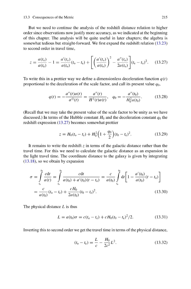
But we need to continue the analysis of the redshift distance relation to higher
order since observations now justify more accuracy, as we indicated at the beginning
of this chapter. The analysis will be quite useful in later chapters; the algebra is
somewhat tedious but straight-forward. We first expand the redshift relation (13.23)
to second order in travel time,
z =
a(t o )
a(t e )
− 1 =
a
(t o )
a(t o )
(t o − t e ) +
a
(t o )
a(t o )
2
−
a
(t o )
2a(t o )
(t e − t o )
2
. (13.27)
To write this in a prettier way we define a dimensionless deceleration function q(t)
proportional to the deceleration of the scale factor, and call its present value q 0 ,
q(t) = −
a
(t)a(t)
a 2 (t)
=
a
(t)
H 2 (t)a(t)
, q 0 = −
a
(t 0 )
H
2
0 a(t 0 )
.
(13.28)
(Recall that we may take the present value of the scale factor to be unity as we have
discussed.) In terms of the Hubble constant H 0 and the deceleration constant q 0 the
redshift expression (13.27) becomes somewhat prettier
z = H 0 (t o − t e ) + H
2
0
1 +
q 0
2
(t 0 − t e )
2
.
(13.29)
It remains to write the redshift z in terms of the galactic distance rather than the
travel time. For this we need to calculate the galactic distance as an expansion in
the light travel time. The coordinate distance to the galaxy is given by integrating
(13.18), so we obtain by expansion
σ =
t 0
t e
cdt
a(t)
=
t 0
t e
cdt
a(t 0 ) + a (t 0 )(t − t o )
=
c
a(t 0 )
t 0
t e
dt
1 −
a
(t 0 )
a(t 0 )
(t − t o )
=
c
a(t 0 )
(t o − t e ) +
cH 0
2a(t 0 )
(t 0 − t e )
2
.
(13.30)
The physical distance L is thus
L = a(t 0 )σ = c(t o − t e ) + cH 0 (t 0 − t e )
2
/2.
(13.31)
Inverting this to second order we get the travel time in terms of the physical distance,
(t o − t e ) =
L
c
−
H 0
2c 2 L
2
.
(13.32)
215
But we need to continue the analysis of the redshift distance relation to higher
order since observations now justify more accuracy, as we indicated at the beginning
of this chapter. The analysis will be quite useful in later chapters; the algebra is
somewhat tedious but straight-forward. We first expand the redshift relation (13.23)
to second order in travel time,
z =
a(t o )
a(t e )
− 1 =
a
(t o )
a(t o )
(t o − t e ) +
a
(t o )
a(t o )
2
−
a
(t o )
2a(t o )
(t e − t o )
2
. (13.27)
To write this in a prettier way we define a dimensionless deceleration function q(t)
proportional to the deceleration of the scale factor, and call its present value q 0 ,
q(t) = −
a
(t)a(t)
a 2 (t)
=
a
(t)
H 2 (t)a(t)
, q 0 = −
a
(t 0 )
H
2
0 a(t 0 )
.
(13.28)
(Recall that we may take the present value of the scale factor to be unity as we have
discussed.) In terms of the Hubble constant H 0 and the deceleration constant q 0 the
redshift expression (13.27) becomes somewhat prettier
z = H 0 (t o − t e ) + H
2
0
1 +
q 0
2
(t 0 − t e )
2
.
(13.29)
It remains to write the redshift z in terms of the galactic distance rather than the
travel time. For this we need to calculate the galactic distance as an expansion in
the light travel time. The coordinate distance to the galaxy is given by integrating
(13.18), so we obtain by expansion
σ =
t 0
t e
cdt
a(t)
=
t 0
t e
cdt
a(t 0 ) + a (t 0 )(t − t o )
=
c
a(t 0 )
t 0
t e
dt
1 −
a
(t 0 )
a(t 0 )
(t − t o )
=
c
a(t 0 )
(t o − t e ) +
cH 0
2a(t 0 )
(t 0 − t e )
2
.
(13.30)
The physical distance L is thus
L = a(t 0 )σ = c(t o − t e ) + cH 0 (t 0 − t e )
2
/2.
(13.31)
Inverting this to second order we get the travel time in terms of the physical distance,
(t o − t e ) =
L
c
−
H 0
2c 2 L
2
.
(13.32)