

216
13 Cosmological Preliminaries
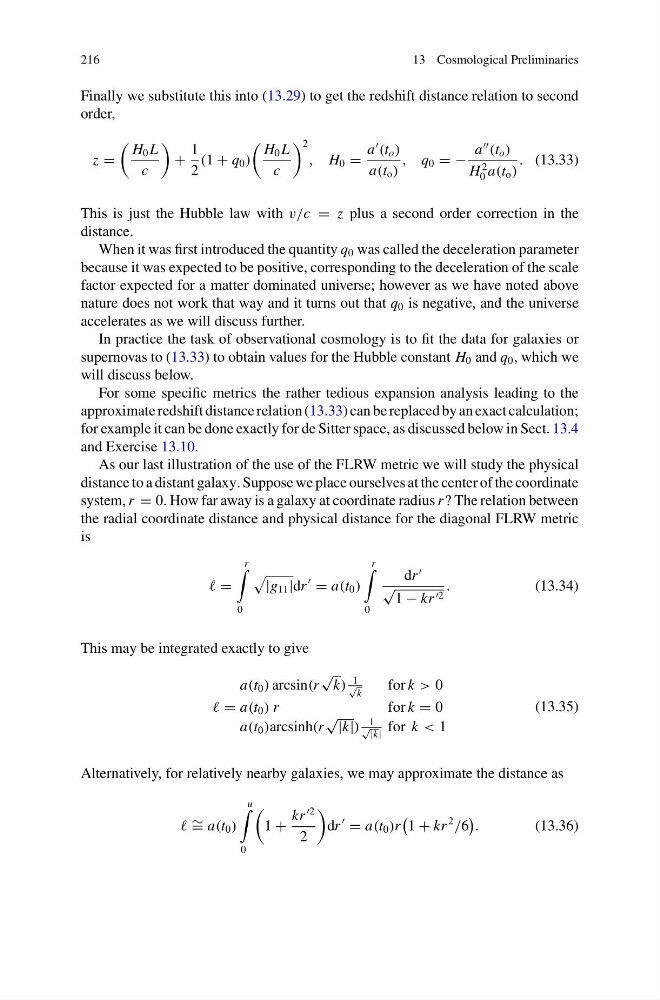
Finally we substitute this into (13.29) to get the redshift distance relation to second
order,
z =
H 0 L
c
+
1
2
(1 + q 0 )
H 0 L
c
2
, H 0 =
a
(t o )
a(t o )
, q 0 = −
a
(t o )
H
2
0 a(t o )
. (13.33)
This is just the Hubble law with v/c = z plus a second order correction in the
distance.
When it was first introduced the quantity q 0 was called the deceleration parameter
because it was expected to be positive, corresponding to the deceleration of the scale
factor expected for a matter dominated universe; however as we have noted above
nature does not work that way and it turns out that q 0 is negative, and the universe
accelerates as we will discuss further.
In practice the task of observational cosmology is to fit the data for galaxies or
supernovas to (13.33) to obtain values for the Hubble constant H 0 and q 0 , which we
will discuss below.
For some specific metrics the rather tedious expansion analysis leading to the
approximate redshift distance relation (13.33) can be replaced by an exact calculation;
for example it can be done exactly for de Sitter space, as discussed below in Sect. 13.4
and Exercise 13.10.
As our last illustration of the use of the FLRW metric we will study the physical
distance to a distant galaxy. Suppose we place ourselves at the center of the coordinate
system, r = 0. How far away is a galaxy at coordinate radius r ? The relation between
the radial coordinate distance and physical distance for the diagonal FLRW metric
is
=
r
0
|g 11 |dr
= a(t 0 )
r
0
dr
√
1 − kr 2
.
(13.34)
This may be integrated exactly to give
a(t 0 ) arcsin(r
√
k)
1
√
k
for k > 0
= a(t 0 ) r
for k = 0
a(t 0 )arcsinh(r
√
|k|)
1
√
|k|
for k < 1
(13.35)
Alternatively, for relatively nearby galaxies, we may approximate the distance as
∼ = a(t 0 )
u
0
1 +
kr
2
2
dr
= a(t 0 )r
1 + kr
2
/6
.
(13.36)
13 Cosmological Preliminaries
Finally we substitute this into (13.29) to get the redshift distance relation to second
order,
z =
H 0 L
c
+
1
2
(1 + q 0 )
H 0 L
c
2
, H 0 =
a
(t o )
a(t o )
, q 0 = −
a
(t o )
H
2
0 a(t o )
. (13.33)
This is just the Hubble law with v/c = z plus a second order correction in the
distance.
When it was first introduced the quantity q 0 was called the deceleration parameter
because it was expected to be positive, corresponding to the deceleration of the scale
factor expected for a matter dominated universe; however as we have noted above
nature does not work that way and it turns out that q 0 is negative, and the universe
accelerates as we will discuss further.
In practice the task of observational cosmology is to fit the data for galaxies or
supernovas to (13.33) to obtain values for the Hubble constant H 0 and q 0 , which we
will discuss below.
For some specific metrics the rather tedious expansion analysis leading to the
approximate redshift distance relation (13.33) can be replaced by an exact calculation;
for example it can be done exactly for de Sitter space, as discussed below in Sect. 13.4
and Exercise 13.10.
As our last illustration of the use of the FLRW metric we will study the physical
distance to a distant galaxy. Suppose we place ourselves at the center of the coordinate
system, r = 0. How far away is a galaxy at coordinate radius r ? The relation between
the radial coordinate distance and physical distance for the diagonal FLRW metric
is
=
r
0
|g 11 |dr
= a(t 0 )
r
0
dr
√
1 − kr 2
.
(13.34)
This may be integrated exactly to give
a(t 0 ) arcsin(r
√
k)
1
√
k
for k > 0
= a(t 0 ) r
for k = 0
a(t 0 )arcsinh(r
√
|k|)
1
√
|k|
for k < 1
(13.35)
Alternatively, for relatively nearby galaxies, we may approximate the distance as
∼ = a(t 0 )
u
0
1 +
kr
2
2
dr
= a(t 0 )r
1 + kr
2
/6
.
(13.36)