

11.1 The Field Equations of the Linearized Theory
161
R
αβγ δ = R αβγ δ .
(11.9)
The situation is in close analogy to gauge invariance in electromagnetism: a gauge
change of the vector potential does not change the electromagnetic fields; the gauge
change of the coordinates does not change the Reimann tensor, which is the intrinsic
indicator of the gravitational field as we discussed in Chap. 8.
The expression f μ,ν + f ν,μ that appears in (11.8) gives a null Riemann tensor
or flat space, and thus must be a solution of the field equations; it is called a Weyl
solution. We will find the idea of gauge transformations and the gauge invariance of
the Reimann tensor very useful when we study gravitational waves.
The Ricci tensor and Riemann (or Ricci) scalar follow from contraction of the
Reimann tensor (11.6). Using the symmetry of the metric and second derivatives and
raising and lowering indices with the Lorentz metric we find for the Ricci tensor and
the Riemann scalar,
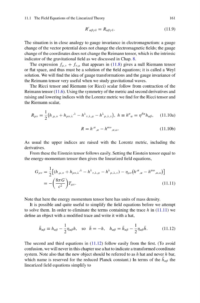
R μν =
1
2
h ,μ,ν + h μν,λ
,λ
− h
λ ν,λ,μ − h
λ μ,λ,ν
, h ≡ h
α α = η
βα h αβ , (11.10a)
R = h
,α ,α − h
αω ,α,ω .
(11.10b)
As usual the upper indices are raised with the Lorentz metric, including the
derivatives.
From these the Einstein tensor follows easily. Setting the Einstein tensor equal to
the energy-momentum tensor then gives the linearized field equations,
G μν =
1
2
(h ,μ,ν + h μν,λ
,λ
− h
λ ν,λ,μ − h
λ μ,λ,ν ) − η μν
h
,α ,α − h
αω ,α,ω
= −
8π G
c 2
T μν .
(11.11)
Note that here the energy momentum tensor here has units of mass density.
It is possible and quite useful to simplify the field equations before we attempt
to solve them. In order to eliminate the terms containing the trace h in (11.11) we
define an object with a modified trace and write it with a hat,
¯
h αβ ≡ h αβ −
1
2
η αβ h, so ¯
h = −h, h αβ = ¯
h αβ −
1
2
η αβ ¯
h.
(11.12)
The second and third equations in (11.12) follow easily from the first. (To avoid
confusion, we will never in this chapter use a hat to indicate a transformed coordinate
system. Note also that the new object should be referred to as h hat and never h bar,
which name is reserved for the reduced Planck constant.) In terms of the ¯
h αβ the
linearized field equations simplify to
161
R
αβγ δ = R αβγ δ .
(11.9)
The situation is in close analogy to gauge invariance in electromagnetism: a gauge
change of the vector potential does not change the electromagnetic fields; the gauge
change of the coordinates does not change the Reimann tensor, which is the intrinsic
indicator of the gravitational field as we discussed in Chap. 8.
The expression f μ,ν + f ν,μ that appears in (11.8) gives a null Riemann tensor
or flat space, and thus must be a solution of the field equations; it is called a Weyl
solution. We will find the idea of gauge transformations and the gauge invariance of
the Reimann tensor very useful when we study gravitational waves.
The Ricci tensor and Riemann (or Ricci) scalar follow from contraction of the
Reimann tensor (11.6). Using the symmetry of the metric and second derivatives and
raising and lowering indices with the Lorentz metric we find for the Ricci tensor and
the Riemann scalar,
R μν =
1
2
h ,μ,ν + h μν,λ
,λ
− h
λ ν,λ,μ − h
λ μ,λ,ν
, h ≡ h
α α = η
βα h αβ , (11.10a)
R = h
,α ,α − h
αω ,α,ω .
(11.10b)
As usual the upper indices are raised with the Lorentz metric, including the
derivatives.
From these the Einstein tensor follows easily. Setting the Einstein tensor equal to
the energy-momentum tensor then gives the linearized field equations,
G μν =
1
2
(h ,μ,ν + h μν,λ
,λ
− h
λ ν,λ,μ − h
λ μ,λ,ν ) − η μν
h
,α ,α − h
αω ,α,ω
= −
8π G
c 2
T μν .
(11.11)
Note that here the energy momentum tensor here has units of mass density.
It is possible and quite useful to simplify the field equations before we attempt
to solve them. In order to eliminate the terms containing the trace h in (11.11) we
define an object with a modified trace and write it with a hat,
¯
h αβ ≡ h αβ −
1
2
η αβ h, so ¯
h = −h, h αβ = ¯
h αβ −
1
2
η αβ ¯
h.
(11.12)
The second and third equations in (11.12) follow easily from the first. (To avoid
confusion, we will never in this chapter use a hat to indicate a transformed coordinate
system. Note also that the new object should be referred to as h hat and never h bar,
which name is reserved for the reduced Planck constant.) In terms of the ¯
h αβ the
linearized field equations simplify to