

160
11 Linearized General Relativity and Gravitational Waves
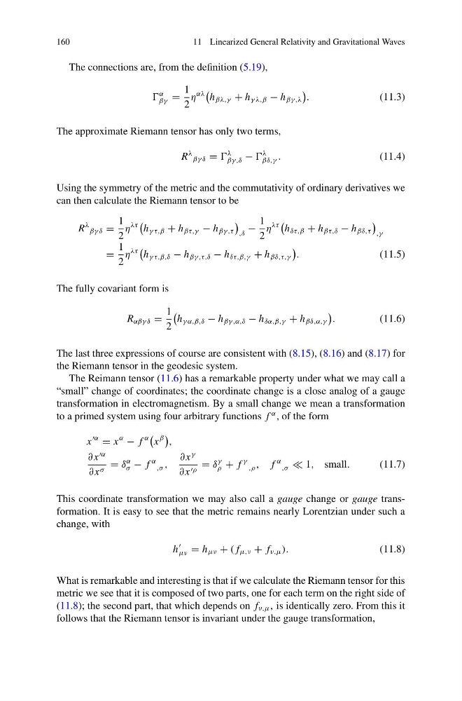
The connections are, from the definition (5.19),
α
βγ =
1
2
η
αλ
h βλ,γ + h γ λ,β − h βγ,λ
.
(11.3)
The approximate Riemann tensor has only two terms,
R
λ βγ δ =
λ
βγ,δ −
λ
βδ,γ .
(11.4)
Using the symmetry of the metric and the commutativity of ordinary derivatives we
can then calculate the Riemann tensor to be
R
λ βγ δ =
1
2
η
λτ
h γ τ,β + h βτ,γ − h βγ,τ
,δ
−
1
2
η
λτ
h δτ,β + h βτ,δ − h βδ,τ
,γ
=
1
2
η
λτ
h γ τ,β,δ − h βγ ,τ,δ − h δτ,β,γ + h βδ,τ,γ
.
(11.5)
The fully covariant form is
R αβγ δ =
1
2
h γ α,β,δ − h βγ ,α,δ − h δα,β,γ + h βδ,α,γ
.
(11.6)
The last three expressions of course are consistent with (8.15), (8.16) and (8.17) for
the Riemann tensor in the geodesic system.
The Reimann tensor (11.6) has a remarkable property under what we may call a
“small” change of coordinates; the coordinate change is a close analog of a gauge
transformation in electromagnetism. By a small change we mean a transformation
to a primed system using four arbitrary functions f
α , of the form
x
α
= x
α
− f
α
x
β
,
∂ x
α
∂ x σ = δ
α
σ − f
α ,σ ,
∂ x
γ
∂ x ρ = δ
γ
ρ + f
γ ,ρ , f
α ,σ 1, small.
(11.7)
This coordinate transformation we may also call a gauge change or gauge transformation. It is easy to see that the metric remains nearly Lorentzian under such a
change, with
h
μν = h μν + ( f μ,ν + f ν,μ ).
(11.8)
What is remarkable and interesting is that if we calculate the Riemann tensor for this
metric we see that it is composed of two parts, one for each term on the right side of
(11.8); the second part, that which depends on f ν,μ , is identically zero. From this it
follows that the Riemann tensor is invariant under the gauge transformation,
11 Linearized General Relativity and Gravitational Waves
The connections are, from the definition (5.19),
α
βγ =
1
2
η
αλ
h βλ,γ + h γ λ,β − h βγ,λ
.
(11.3)
The approximate Riemann tensor has only two terms,
R
λ βγ δ =
λ
βγ,δ −
λ
βδ,γ .
(11.4)
Using the symmetry of the metric and the commutativity of ordinary derivatives we
can then calculate the Riemann tensor to be
R
λ βγ δ =
1
2
η
λτ
h γ τ,β + h βτ,γ − h βγ,τ
,δ
−
1
2
η
λτ
h δτ,β + h βτ,δ − h βδ,τ
,γ
=
1
2
η
λτ
h γ τ,β,δ − h βγ ,τ,δ − h δτ,β,γ + h βδ,τ,γ
.
(11.5)
The fully covariant form is
R αβγ δ =
1
2
h γ α,β,δ − h βγ ,α,δ − h δα,β,γ + h βδ,α,γ
.
(11.6)
The last three expressions of course are consistent with (8.15), (8.16) and (8.17) for
the Riemann tensor in the geodesic system.
The Reimann tensor (11.6) has a remarkable property under what we may call a
“small” change of coordinates; the coordinate change is a close analog of a gauge
transformation in electromagnetism. By a small change we mean a transformation
to a primed system using four arbitrary functions f
α , of the form
x
α
= x
α
− f
α
x
β
,
∂ x
α
∂ x σ = δ
α
σ − f
α ,σ ,
∂ x
γ
∂ x ρ = δ
γ
ρ + f
γ ,ρ , f
α ,σ 1, small.
(11.7)
This coordinate transformation we may also call a gauge change or gauge transformation. It is easy to see that the metric remains nearly Lorentzian under such a
change, with
h
μν = h μν + ( f μ,ν + f ν,μ ).
(11.8)
What is remarkable and interesting is that if we calculate the Riemann tensor for this
metric we see that it is composed of two parts, one for each term on the right side of
(11.8); the second part, that which depends on f ν,μ , is identically zero. From this it
follows that the Riemann tensor is invariant under the gauge transformation,