

234
C. McCammon
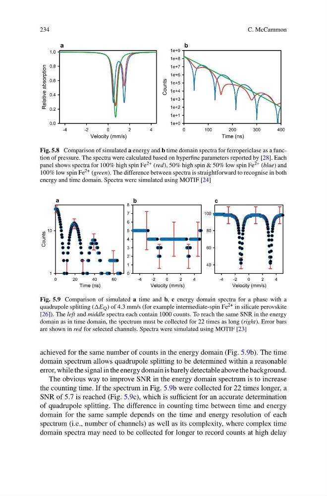
Fig. 5.8 Comparison of simulated a energy and b time domain spectra for ferropericlase as a function of pressure. The spectra were calculated based on hyperfine parameters reported by [28]. Each
panel shows spectra for 100% high spin Fe 2+ (red), 50% high spin & 50% low spin Fe 2+ (blue) and
100% low spin Fe 2+ (green). The difference between spectra is straightforward to recognise in both
energy and time domain. Spectra were simulated using MOTIF [24]
Fig. 5.9 Comparison of simulated a time and b, c energy domain spectra for a phase with a
quadrupole splitting ( Q ) of 4.3 mm/s (for example intermediate-spin Fe 2+ in silicate perovskite
[26]). The left and middle spectra each contain 1000 counts. To reach the same SNR in the energy
domain as in time domain, the spectrum must be collected for 22 times as long (right). Error bars
are shown in red for selected channels. Spectra were simulated using MOTIF [23]
achieved for the same number of counts in the energy domain (Fig. 5.9b). The time
domain spectrum allows quadrupole splitting to be determined within a reasonable
error, while the signal in the energy domain is barely detectable above the background.
The obvious way to improve SNR in the energy domain spectrum is to increase
the counting time. If the spectrum in Fig. 5.9b were collected for 22 times longer, a
SNR of 5.7 is reached (Fig. 5.9c), which is sufficient for an accurate determination
of quadrupole splitting. The difference in counting time between time and energy
domain for the same sample depends on the time and energy resolution of each
spectrum (i.e., number of channels) as well as its complexity, where complex time
domain spectra may need to be collected for longer to record counts at high delay
C. McCammon
Fig. 5.8 Comparison of simulated a energy and b time domain spectra for ferropericlase as a function of pressure. The spectra were calculated based on hyperfine parameters reported by [28]. Each
panel shows spectra for 100% high spin Fe 2+ (red), 50% high spin & 50% low spin Fe 2+ (blue) and
100% low spin Fe 2+ (green). The difference between spectra is straightforward to recognise in both
energy and time domain. Spectra were simulated using MOTIF [24]
Fig. 5.9 Comparison of simulated a time and b, c energy domain spectra for a phase with a
quadrupole splitting ( Q ) of 4.3 mm/s (for example intermediate-spin Fe 2+ in silicate perovskite
[26]). The left and middle spectra each contain 1000 counts. To reach the same SNR in the energy
domain as in time domain, the spectrum must be collected for 22 times as long (right). Error bars
are shown in red for selected channels. Spectra were simulated using MOTIF [23]
achieved for the same number of counts in the energy domain (Fig. 5.9b). The time
domain spectrum allows quadrupole splitting to be determined within a reasonable
error, while the signal in the energy domain is barely detectable above the background.
The obvious way to improve SNR in the energy domain spectrum is to increase
the counting time. If the spectrum in Fig. 5.9b were collected for 22 times longer, a
SNR of 5.7 is reached (Fig. 5.9c), which is sufficient for an accurate determination
of quadrupole splitting. The difference in counting time between time and energy
domain for the same sample depends on the time and energy resolution of each
spectrum (i.e., number of channels) as well as its complexity, where complex time
domain spectra may need to be collected for longer to record counts at high delay