

5 Mössbauer Spectroscopy with High Spatial Resolution …
233
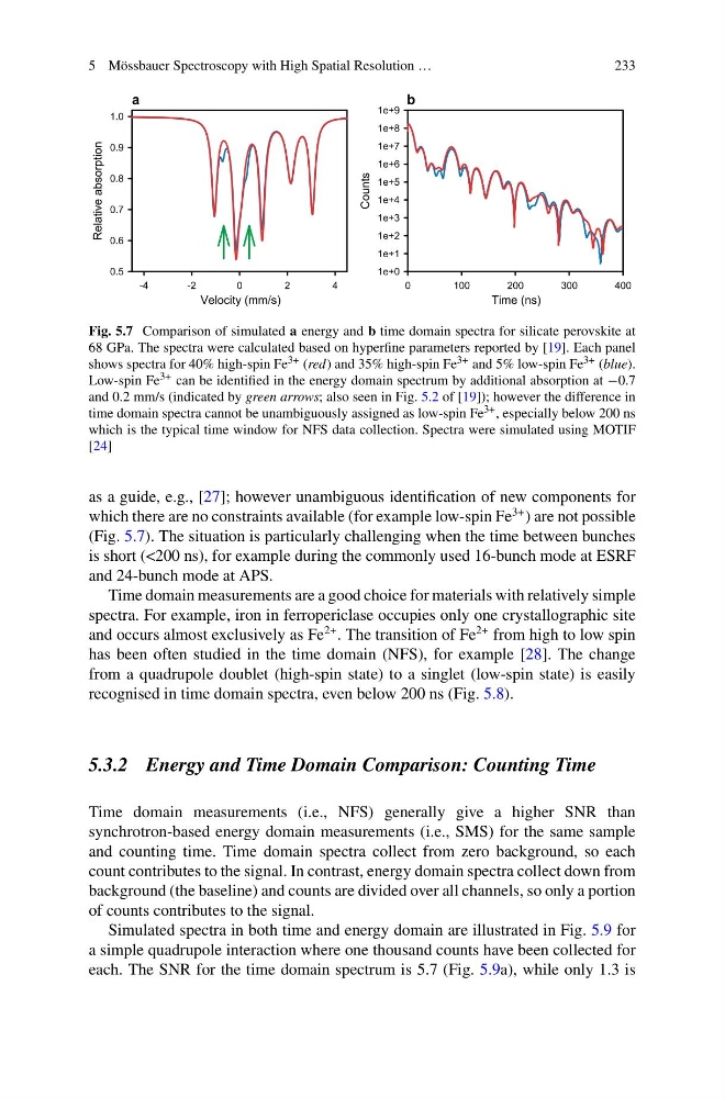
Fig. 5.7 Comparison of simulated a energy and b time domain spectra for silicate perovskite at
68 GPa. The spectra were calculated based on hyperfine parameters reported by [19]. Each panel
shows spectra for 40% high-spin Fe 3+ (red) and 35% high-spin Fe 3+ and 5% low-spin Fe 3+ (blue).
Low-spin Fe 3+ can be identified in the energy domain spectrum by additional absorption at −0.7
and 0.2 mm/s (indicated by green arrows; also seen in Fig. 5.2 of [19]); however the difference in
time domain spectra cannot be unambiguously assigned as low-spin Fe 3+ , especially below 200 ns
which is the typical time window for NFS data collection. Spectra were simulated using MOTIF
[24]
as a guide, e.g., [27]; however unambiguous identification of new components for
which there are no constraints available (for example low-spin Fe
3+ ) are not possible
(Fig. 5.7). The situation is particularly challenging when the time between bunches
is short (<200 ns), for example during the commonly used 16-bunch mode at ESRF
and 24-bunch mode at APS.
Time domain measurements are a good choice for materials with relatively simple
spectra. For example, iron in ferropericlase occupies only one crystallographic site
and occurs almost exclusively as Fe
2+ . The transition of Fe
2+ from high to low spin
has been often studied in the time domain (NFS), for example [28]. The change
from a quadrupole doublet (high-spin state) to a singlet (low-spin state) is easily
recognised in time domain spectra, even below 200 ns (Fig. 5.8).
5.3.2 Energy and Time Domain Comparison: Counting Time
Time domain measurements (i.e., NFS) generally give a higher SNR than
synchrotron-based energy domain measurements (i.e., SMS) for the same sample
and counting time. Time domain spectra collect from zero background, so each
count contributes to the signal. In contrast, energy domain spectra collect down from
background (the baseline) and counts are divided over all channels, so only a portion
of counts contributes to the signal.
Simulated spectra in both time and energy domain are illustrated in Fig. 5.9 for
a simple quadrupole interaction where one thousand counts have been collected for
each. The SNR for the time domain spectrum is 5.7 (Fig. 5.9a), while only 1.3 is
233
Fig. 5.7 Comparison of simulated a energy and b time domain spectra for silicate perovskite at
68 GPa. The spectra were calculated based on hyperfine parameters reported by [19]. Each panel
shows spectra for 40% high-spin Fe 3+ (red) and 35% high-spin Fe 3+ and 5% low-spin Fe 3+ (blue).
Low-spin Fe 3+ can be identified in the energy domain spectrum by additional absorption at −0.7
and 0.2 mm/s (indicated by green arrows; also seen in Fig. 5.2 of [19]); however the difference in
time domain spectra cannot be unambiguously assigned as low-spin Fe 3+ , especially below 200 ns
which is the typical time window for NFS data collection. Spectra were simulated using MOTIF
[24]
as a guide, e.g., [27]; however unambiguous identification of new components for
which there are no constraints available (for example low-spin Fe
3+ ) are not possible
(Fig. 5.7). The situation is particularly challenging when the time between bunches
is short (<200 ns), for example during the commonly used 16-bunch mode at ESRF
and 24-bunch mode at APS.
Time domain measurements are a good choice for materials with relatively simple
spectra. For example, iron in ferropericlase occupies only one crystallographic site
and occurs almost exclusively as Fe
2+ . The transition of Fe
2+ from high to low spin
has been often studied in the time domain (NFS), for example [28]. The change
from a quadrupole doublet (high-spin state) to a singlet (low-spin state) is easily
recognised in time domain spectra, even below 200 ns (Fig. 5.8).
5.3.2 Energy and Time Domain Comparison: Counting Time
Time domain measurements (i.e., NFS) generally give a higher SNR than
synchrotron-based energy domain measurements (i.e., SMS) for the same sample
and counting time. Time domain spectra collect from zero background, so each
count contributes to the signal. In contrast, energy domain spectra collect down from
background (the baseline) and counts are divided over all channels, so only a portion
of counts contributes to the signal.
Simulated spectra in both time and energy domain are illustrated in Fig. 5.9 for
a simple quadrupole interaction where one thousand counts have been collected for
each. The SNR for the time domain spectrum is 5.7 (Fig. 5.9a), while only 1.3 is