

Study on Material Point Method with Different Influence Factors
79
3.3 Shock Temperature
Shock temperature is an important parameter during the process of impact compression
analysis [13]. It can be obtained by thermodynamic function, conservation equation and
Hugoniot curve.
There are three methods to obtain the shock temperature [14–18]: 1. Obtained from
Gruneisen state equation and Hugoniot curve; 2. Obtained from three-term equation of
state; 3. Obtained from Gruneisen state equation which is taken the isentropic line as
the reference line. According to the conclusions analyzed by Tang [19], the first method
has the least parameters to compute the shock temperature but it does not consider the
influence of phase change. The second method has the most comprehensive considerations and it has the most parameters to compute the shock temperature. The last method
is related to the isentropic line which means that the accuracy of the computed shock
temperature depends on the choice of the isentropic equation. Compared the computed
shock temperature to the test, the results show that the second method has a good result
in both solid phase and liquid phase while the first method has a good result in solid
phase only. We do not consider liquid phase in this paper and the first method has the
least considered parameters. Hence, the first method is taken as the method to obtain the
shock temperature in MPM algorithm.
According to the thermodynamic functions,
de + pdv = c v dT +
(δe/δv) T + p
dv
(10)
p + (δe/δv) T = T (δS/δv) T = Tc v γ /v
(11)
Equation (12) can be derived,
de + pdv = c v dT + Tc v (γ /v)dv
(12)
Where c v is the material’s specific heat at a constant volume. γ is the parameter of
Gruneisen. v is the specific volume and e is the specific internal energy.
Combination of the Eq. (12) with the parameters of the Hugoniot curve,
dT H
dv
+
γ
v
T H =
1
2c v
p H + (v 0 − v)(dp H /dv)
dv
(13)
Where the subscript H stands for the parameters which are under the state of Hugoniot
curve. The subscript 0 stands for the parameters which are under the state of zeropressure. γ is ensured by the equation
γ
v
=
γ 0
v 0
(14)
η =
μ
1 + μ
(15)
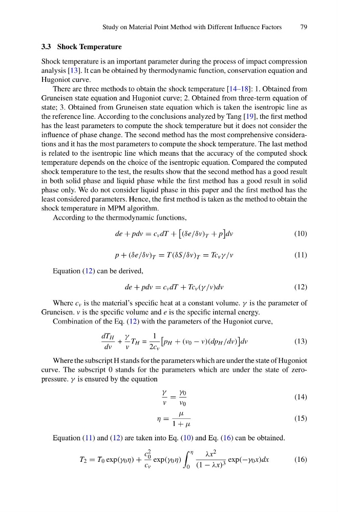
Equation (11) and (12) are taken into Eq. (10) and Eq. (16) can be obtained.
T 2 = T 0 exp(γ 0 η) +
c 2
0
c v
exp(γ 0 η)
η
0
λx 2
(1 − λx) 3 exp(−γ 0 x)dx
(16)
79
3.3 Shock Temperature
Shock temperature is an important parameter during the process of impact compression
analysis [13]. It can be obtained by thermodynamic function, conservation equation and
Hugoniot curve.
There are three methods to obtain the shock temperature [14–18]: 1. Obtained from
Gruneisen state equation and Hugoniot curve; 2. Obtained from three-term equation of
state; 3. Obtained from Gruneisen state equation which is taken the isentropic line as
the reference line. According to the conclusions analyzed by Tang [19], the first method
has the least parameters to compute the shock temperature but it does not consider the
influence of phase change. The second method has the most comprehensive considerations and it has the most parameters to compute the shock temperature. The last method
is related to the isentropic line which means that the accuracy of the computed shock
temperature depends on the choice of the isentropic equation. Compared the computed
shock temperature to the test, the results show that the second method has a good result
in both solid phase and liquid phase while the first method has a good result in solid
phase only. We do not consider liquid phase in this paper and the first method has the
least considered parameters. Hence, the first method is taken as the method to obtain the
shock temperature in MPM algorithm.
According to the thermodynamic functions,
de + pdv = c v dT +
(δe/δv) T + p
dv
(10)
p + (δe/δv) T = T (δS/δv) T = Tc v γ /v
(11)
Equation (12) can be derived,
de + pdv = c v dT + Tc v (γ /v)dv
(12)
Where c v is the material’s specific heat at a constant volume. γ is the parameter of
Gruneisen. v is the specific volume and e is the specific internal energy.
Combination of the Eq. (12) with the parameters of the Hugoniot curve,
dT H
dv
+
γ
v
T H =
1
2c v
p H + (v 0 − v)(dp H /dv)
dv
(13)
Where the subscript H stands for the parameters which are under the state of Hugoniot
curve. The subscript 0 stands for the parameters which are under the state of zeropressure. γ is ensured by the equation
γ
v
=
γ 0
v 0
(14)
η =
μ
1 + μ
(15)
Equation (11) and (12) are taken into Eq. (10) and Eq. (16) can be obtained.
T 2 = T 0 exp(γ 0 η) +
c 2
0
c v
exp(γ 0 η)
η
0
λx 2
(1 − λx) 3 exp(−γ 0 x)dx
(16)