

Nonreflecting Outlet Boundary Conditions for Smoothed Particle Hydrodynamics
67
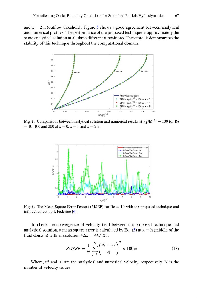
and x = 2 h (outflow threshold). Figure 5 shows a good agreement between analytical
and numerical profiles. The performance of the proposed technique is approximately the
same analytical solution at all three different x-positions. Therefore, it demonstrates the
stability of this technique throughout the computational domain.
Fig. 5. Comparisons between analytical solution and numerical results at t(g/h) 1/2 = 100 for Re
= 10, 100 and 200 at x = 0, x = h and x = 2 h.
Fig. 6. The Mean Square Error Percent (MSEP) for Re = 10 with the proposed technique and
inflow/outflow by I. Federico [6]
To check the convergence of velocity field between the proposed technique and
analytical solution, a mean square error is calculated by Eq. (5) at x = h (middle of the
fluid domain) with a resolution 4x = 4h/125.
RMSEP =
1
N
N
j=1
u a
j − u n
j
u a
j
2
× 100%
(13)
Where, u a and u n are the analytical and numerical velocity, respectively. N is the
number of velocity values.
67
and x = 2 h (outflow threshold). Figure 5 shows a good agreement between analytical
and numerical profiles. The performance of the proposed technique is approximately the
same analytical solution at all three different x-positions. Therefore, it demonstrates the
stability of this technique throughout the computational domain.
Fig. 5. Comparisons between analytical solution and numerical results at t(g/h) 1/2 = 100 for Re
= 10, 100 and 200 at x = 0, x = h and x = 2 h.
Fig. 6. The Mean Square Error Percent (MSEP) for Re = 10 with the proposed technique and
inflow/outflow by I. Federico [6]
To check the convergence of velocity field between the proposed technique and
analytical solution, a mean square error is calculated by Eq. (5) at x = h (middle of the
fluid domain) with a resolution 4x = 4h/125.
RMSEP =
1
N
N
j=1
u a
j − u n
j
u a
j
2
× 100%
(13)
Where, u a and u n are the analytical and numerical velocity, respectively. N is the
number of velocity values.