

290
Y. Xu et al.
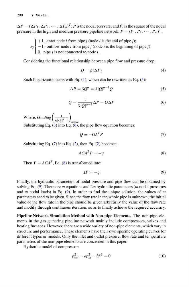
P = (P 1 , ,P 2 , · · · , ,P n )
T ; P is the nodal pressure, and P i is the square of the nodal
pressure in the high and medium pressure pipeline network, P = (P 1 , P 2 , · · · , P m )
T .
a ij
⎧
⎨
⎩
+1, enter node i from pipe j (node i is the end of pipe j);
−1, outflow node i from pipe j (node i is the beginning of pipe j);
0, pipe j is not connected to node i.
Considering the functional relationship between pipe flow and pressure drop:
Q = φ(P)
(4)
Such linearization starts with Eq. (1), which can be rewritten as Eq. (5):
P = SQ
α
= S|Q|
α−1 Q
(5)
Q =
1
S|Q|
α−1
P = GP
(6)
Where, G=diag
1
s j |Qj|
α−1
m×m
Substituting Eq. (3) into Eq. (6), the pipe flow equation becomes:
Q = −GA
T P
(7)
Substituting Eq. (7) into Eq. (2), then Eq. (2) becomes:
AGA
T P = −q
(8)
Then Y = AGA T , Eq. (8) is transformed into:
YP = −q
(9)
Finally, the hydraulic parameters of nodal pressure and pipe flow can be obtained by
solving Eq. (9). There are m equations and 2m hydraulic parameters (m nodal pressures
and m nodal loads) in Eq. (9). In order to find the unique solution, the values of m
parameters need to be given. Since the flow rate in the whole pipe is unknown, the initial
value of the flow rate in the pipe should be given arbitrarily the value of the flow rate
and modify through continuous iteration, so as to finally achieve the required accuracy.
Pipeline Network Simulation Method with Non-pipe Elements. The non-pipe elements in the gas gathering pipeline network mainly include compressors, valves and
heating furnaces. However, there are a wide variety of non-pipe elements, which vary in
structure and performance. These elements have their own specific operating curves for
different types or models. Only the inlet and outlet pressure, flow rate and temperature
parameters of the non-pipe elements are concerned in this paper.
Hydraulic model of compressor:
p
2
out − ap
2
in − bf
2
= 0
( 1 0 )
Y. Xu et al.
P = (P 1 , ,P 2 , · · · , ,P n )
T ; P is the nodal pressure, and P i is the square of the nodal
pressure in the high and medium pressure pipeline network, P = (P 1 , P 2 , · · · , P m )
T .
a ij
⎧
⎨
⎩
+1, enter node i from pipe j (node i is the end of pipe j);
−1, outflow node i from pipe j (node i is the beginning of pipe j);
0, pipe j is not connected to node i.
Considering the functional relationship between pipe flow and pressure drop:
Q = φ(P)
(4)
Such linearization starts with Eq. (1), which can be rewritten as Eq. (5):
P = SQ
α
= S|Q|
α−1 Q
(5)
Q =
1
S|Q|
α−1
P = GP
(6)
Where, G=diag
1
s j |Qj|
α−1
m×m
Substituting Eq. (3) into Eq. (6), the pipe flow equation becomes:
Q = −GA
T P
(7)
Substituting Eq. (7) into Eq. (2), then Eq. (2) becomes:
AGA
T P = −q
(8)
Then Y = AGA T , Eq. (8) is transformed into:
YP = −q
(9)
Finally, the hydraulic parameters of nodal pressure and pipe flow can be obtained by
solving Eq. (9). There are m equations and 2m hydraulic parameters (m nodal pressures
and m nodal loads) in Eq. (9). In order to find the unique solution, the values of m
parameters need to be given. Since the flow rate in the whole pipe is unknown, the initial
value of the flow rate in the pipe should be given arbitrarily the value of the flow rate
and modify through continuous iteration, so as to finally achieve the required accuracy.
Pipeline Network Simulation Method with Non-pipe Elements. The non-pipe elements in the gas gathering pipeline network mainly include compressors, valves and
heating furnaces. However, there are a wide variety of non-pipe elements, which vary in
structure and performance. These elements have their own specific operating curves for
different types or models. Only the inlet and outlet pressure, flow rate and temperature
parameters of the non-pipe elements are concerned in this paper.
Hydraulic model of compressor:
p
2
out − ap
2
in − bf
2
= 0
( 1 0 )